

the data to the midpoint–time plane. Migration (Section 3.3.7)
in the midpoint–time plane seeks to eliminate artifacts due to
diffractions and convert the seismic section to an image of the
subsurface. The migrated section can then be converted, using
assumptions about velocities, to a depth section. The depth
section is then interpreted together with geological data and
other types of geophysical data, in some cases from drill holes,
to understand the subsurface geology.
This discussion of the processing sequence brings out the
point that although it is natural to treat a seismic section as an
accurate image of the subsurface, it is actually a display of a
seismic wave field showing the energy arriving as a function of
two-way travel time. Thus the quantity shown, vertical displacement or pressure, need not correspond to any geological
reflector of interest. Large arrivals can result from interference
between reflections from small impedance contrasts. Moreover, because a seismic section has been produced by mathematical operations, rather than the physical experiment it
simulates, noise in the data and errors in the processing can
produce spurious artifacts. For example, the conversion of time
to depth is only as accurate as the velocities found by stacking
or otherwise, perhaps from measurements in a drill hole.
As we have seen in discussing migration, seismic sections
are most likely to deviate from the desired images when the
medium has significant lateral variations. For example, a
medium with random heterogeneities can yield spurious short
layered segments, because the reflected energy depends on the
vertical changes in impedance. Thus long-wavelength vertical
variations in impedance are suppressed, whereas both shortand long-wavelength horizontal variations are preserved, and
so can yield a structure with apparent horizontal layering. This
effect can be viewed as a velocity filter (Section 3.3.5) that
reduces horizontal resolution for structures with steep dips.
Similar effects, which are prone to occur at large offsets, may
contribute to the horizontally discontinuous layering observed
in deep crustal reflection data (Section 3.2.4). Hence, as we
will see in various contexts throughout our discussions (e.g.,
Section 7.3), studying three-dimensional velocity structure is
an interesting and challenging enterprise.
3.4 Seismic waves in a spherical earth
In the previous sections, we developed the theory to use the
travel times of seismic waves to study the velocity structure of a
medium composed of flat layers. This analysis is useful when
the ray paths between the source and the receiver are short
enough that the earth’s curvature can be neglected. Because this
is the case for distances less than a few hundred kilometers,
such analysis is used to study structure in the crust and the
uppermost mantle. In this section we develop the corresponding theory for a spherical earth, which can be used for greater
distances and thus greater depths. Application of these results,
discussed in the next section, is our primary tool for studying
the structure of the deep earth.
3.4 Seismic waves in a spherical earth 157
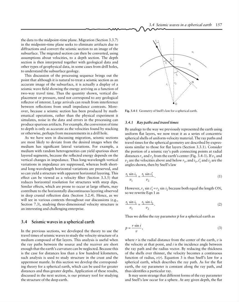
Fig. 3.4-1 Geometry of Snell’s law for a spherical earth.
N
v 1
v 2
i 2
i′ 1
i 2
r 2
r 1
i 1
O
3.4.1 Ray paths and travel times
By analogy to the way we previously represented the earth using
uniform flat layers, we now treat it as a series of concentric
spherical shells of uniform-velocity material. The ray paths and
travel times for the spherical geometry are described by expressions similar to those for flat layers (Section 3.3.1). Consider
the portion of a seismic ray’s path connecting points at radial
distances r 1 and r 2 from the earth’s center (Fig. 3.4-1). If v 1 and
v 2 are the velocities above and below r 1 , and i 1 , i′ 1 and i 2 are the
angles shown, then by Snell’s law
r
i
v
r
i
v
1
1
1
1
1
2
sin
sin .
=
′
(1)
However, r 1 sin i′ 1 = r 2 sin i 2 because both equal the length ON,
so we rewrite Eqn 1 as
r
i
v
r
i
v
1
1
1
2
2
2
sin
sin .
=
(2)
Thus we define the ray parameter p for a spherical earth as
p
r
i
v
sin ,
=
(3)
where r is the radial distance from the center of the earth, v is
the velocity at that point, and i is the incidence angle between
the ray path and the radius vector. By reducing the thickness
of the shells ever thinner, the velocity becomes a continuous
function of radius, v(r). Equation 3 is thus Snell’s law for a
spherical earth, which describes the ray path. As for the flat
earth, the ray parameter is constant along the ray path, and
thus identifies a particular ray.
It may seem strange that different forms of the ray parameter
and Snell’s law occur for a sphere. At any given depth, the flat
in the midpoint–time plane seeks to eliminate artifacts due to
diffractions and convert the seismic section to an image of the
subsurface. The migrated section can then be converted, using
assumptions about velocities, to a depth section. The depth
section is then interpreted together with geological data and
other types of geophysical data, in some cases from drill holes,
to understand the subsurface geology.
This discussion of the processing sequence brings out the
point that although it is natural to treat a seismic section as an
accurate image of the subsurface, it is actually a display of a
seismic wave field showing the energy arriving as a function of
two-way travel time. Thus the quantity shown, vertical displacement or pressure, need not correspond to any geological
reflector of interest. Large arrivals can result from interference
between reflections from small impedance contrasts. Moreover, because a seismic section has been produced by mathematical operations, rather than the physical experiment it
simulates, noise in the data and errors in the processing can
produce spurious artifacts. For example, the conversion of time
to depth is only as accurate as the velocities found by stacking
or otherwise, perhaps from measurements in a drill hole.
As we have seen in discussing migration, seismic sections
are most likely to deviate from the desired images when the
medium has significant lateral variations. For example, a
medium with random heterogeneities can yield spurious short
layered segments, because the reflected energy depends on the
vertical changes in impedance. Thus long-wavelength vertical
variations in impedance are suppressed, whereas both shortand long-wavelength horizontal variations are preserved, and
so can yield a structure with apparent horizontal layering. This
effect can be viewed as a velocity filter (Section 3.3.5) that
reduces horizontal resolution for structures with steep dips.
Similar effects, which are prone to occur at large offsets, may
contribute to the horizontally discontinuous layering observed
in deep crustal reflection data (Section 3.2.4). Hence, as we
will see in various contexts throughout our discussions (e.g.,
Section 7.3), studying three-dimensional velocity structure is
an interesting and challenging enterprise.
3.4 Seismic waves in a spherical earth
In the previous sections, we developed the theory to use the
travel times of seismic waves to study the velocity structure of a
medium composed of flat layers. This analysis is useful when
the ray paths between the source and the receiver are short
enough that the earth’s curvature can be neglected. Because this
is the case for distances less than a few hundred kilometers,
such analysis is used to study structure in the crust and the
uppermost mantle. In this section we develop the corresponding theory for a spherical earth, which can be used for greater
distances and thus greater depths. Application of these results,
discussed in the next section, is our primary tool for studying
the structure of the deep earth.
3.4 Seismic waves in a spherical earth 157
Fig. 3.4-1 Geometry of Snell’s law for a spherical earth.
N
v 1
v 2
i 2
i′ 1
i 2
r 2
r 1
i 1
O
3.4.1 Ray paths and travel times
By analogy to the way we previously represented the earth using
uniform flat layers, we now treat it as a series of concentric
spherical shells of uniform-velocity material. The ray paths and
travel times for the spherical geometry are described by expressions similar to those for flat layers (Section 3.3.1). Consider
the portion of a seismic ray’s path connecting points at radial
distances r 1 and r 2 from the earth’s center (Fig. 3.4-1). If v 1 and
v 2 are the velocities above and below r 1 , and i 1 , i′ 1 and i 2 are the
angles shown, then by Snell’s law
r
i
v
r
i
v
1
1
1
1
1
2
sin
sin .
=
′
(1)
However, r 1 sin i′ 1 = r 2 sin i 2 because both equal the length ON,
so we rewrite Eqn 1 as
r
i
v
r
i
v
1
1
1
2
2
2
sin
sin .
=
(2)
Thus we define the ray parameter p for a spherical earth as
p
r
i
v
sin ,
=
(3)
where r is the radial distance from the center of the earth, v is
the velocity at that point, and i is the incidence angle between
the ray path and the radius vector. By reducing the thickness
of the shells ever thinner, the velocity becomes a continuous
function of radius, v(r). Equation 3 is thus Snell’s law for a
spherical earth, which describes the ray path. As for the flat
earth, the ray parameter is constant along the ray path, and
thus identifies a particular ray.
It may seem strange that different forms of the ray parameter
and Snell’s law occur for a sphere. At any given depth, the flat