

156 Seismology and Earth Structure
waves. Because z increases downward, upcoming waves occur
when k z and ω have the same sign. To ensure this, we define k z
as a function of ω,
k
k
v
k
z
x
x
( , ) sgn ( )
/
,
ω
ω ω
=
−
2 2
2
(79)
where the function sgn (ω) is 1 when ω is positive, and is −1
when ω is negative. Using this definition, the inverse transform
Eqn 73 becomes
u(x, z, t) =
1
4 2
π Ύ Ύ
−∞
∞
−∞
∞
U(k x , 0, ω) exp [i(ωt − k x x
+ k z (ω, k x )z)]dk x dω.
(80)
This integral relates the Fourier transform of the seismic
section recorded on the surface, z = 0, U(k x , 0, ω), and the
upcoming wave field at depth at earlier times. By the exploding
reflector model, the image of the subsurface is the wave field at
t = 0, when the reflectors have just exploded. Thus the image
can be found by setting t = 0:
u(x, z, 0) =
1
4 2
π Ύ Ύ
−∞
∞
−∞
∞
U(k x , 0, ω) exp [i(−k x x
+ k z (ω, k x )z)]dk x dω.
(81)
Although this integral migrates the transform of the seismic
section into the desired image, the integral over ω and k x has to
be done separately to find the image at every depth z. A way to
get around this is to replace the ω integration with one over k z ,
by expressing ω as a function of k x and k z ,
ω( , ) sgn ( )
,
k k
k v k
k
x
z
z
x
z
=
+
2
2
(82)
and changing variables using
d
dk
k v
k
k
z
z
x
z
ω
.
=
+
2
2
(83)
This change converts Eqn 81 into an inverse Fourier transform
from the wavenumber (k x , k z ) domain to the space (x, z) domain
u(x, z, 0) =
1
4 2
π Ύ Ύ
−∞
∞
−∞
∞
U(k x , 0, ω(k x , k z )) exp [i(−k x x
+ k z z)]
k v
k
k
z
x
z
2
2
+
dk x dk z ,
(84)
so inverting the double transform once gives the image for all
x and z.
The application of migration methods to data involves various complexities. The time axis in the section can be scaled
to account for the variation in velocity with depth. Often in
complex geology horizontal variations in velocity are important, so migration can be conducted with numerical methods
that can propagate waves through laterally varying media.
3.3.8 Data processing sequence
The various processing operations for seismic reflection data
can be combined in different ways. To illustrate this, we summarize a common sequence for some of the possible operations.
For simplicity, the discussion is in terms of one horizontal
dimension, but the approach applies to two dimensions.
Preprocessing consists of initial steps. Because data from different receivers are recorded simultaneously, they are reorganized (demultiplexed) to produce a trace for each receiver. The
traces are then edited to eliminate effects such as noisy traces
or recording errors. Static time shifts are applied when needed
(Section 3.3.5). The amplitudes are then adjusted using a gain
recovery function that corrects for the fact that the later arrivals
have lower amplitudes because of reflections, transmissions,
geometric spreading, and attenuation (Section 3.7). The data
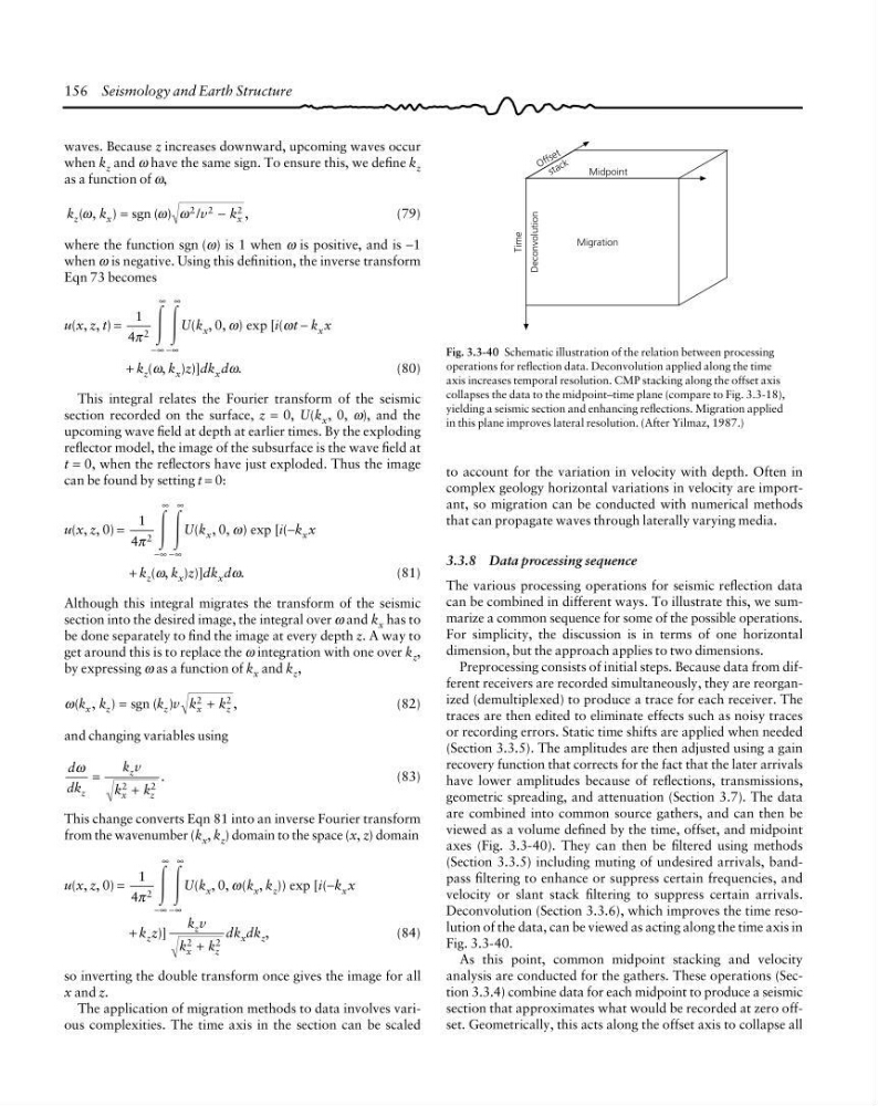
are combined into common source gathers, and can then be
viewed as a volume defined by the time, offset, and midpoint
axes (Fig. 3.3-40). They can then be filtered using methods
(Section 3.3.5) including muting of undesired arrivals, bandpass filtering to enhance or suppress certain frequencies, and
velocity or slant stack filtering to suppress certain arrivals.
Deconvolution (Section 3.3.6), which improves the time resolution of the data, can be viewed as acting along the time axis in
Fig. 3.3-40.
As this point, common midpoint stacking and velocity
analysis are conducted for the gathers. These operations (Section 3.3.4) combine data for each midpoint to produce a seismic
section that approximates what would be recorded at zero offset. Geometrically, this acts along the offset axis to collapse all
Fig. 3.3-40 Schematic illustration of the relation between processing
operations for reflection data. Deconvolution applied along the time
axis increases temporal resolution. CMP stacking along the offset axis
collapses the data to the midpoint–time plane (compare to Fig. 3.3-18),
yielding a seismic section and enhancing reflections. Migration applied
in this plane improves lateral resolution. (After Yilmaz, 1987.)
Migration
s t a c k
O f f s e t
Deconvolution
Time
Midpoint
waves. Because z increases downward, upcoming waves occur
when k z and ω have the same sign. To ensure this, we define k z
as a function of ω,
k
k
v
k
z
x
x
( , ) sgn ( )
/
,
ω
ω ω
=
−
2 2
2
(79)
where the function sgn (ω) is 1 when ω is positive, and is −1
when ω is negative. Using this definition, the inverse transform
Eqn 73 becomes
u(x, z, t) =
1
4 2
π Ύ Ύ
−∞
∞
−∞
∞
U(k x , 0, ω) exp [i(ωt − k x x
+ k z (ω, k x )z)]dk x dω.
(80)
This integral relates the Fourier transform of the seismic
section recorded on the surface, z = 0, U(k x , 0, ω), and the
upcoming wave field at depth at earlier times. By the exploding
reflector model, the image of the subsurface is the wave field at
t = 0, when the reflectors have just exploded. Thus the image
can be found by setting t = 0:
u(x, z, 0) =
1
4 2
π Ύ Ύ
−∞
∞
−∞
∞
U(k x , 0, ω) exp [i(−k x x
+ k z (ω, k x )z)]dk x dω.
(81)
Although this integral migrates the transform of the seismic
section into the desired image, the integral over ω and k x has to
be done separately to find the image at every depth z. A way to
get around this is to replace the ω integration with one over k z ,
by expressing ω as a function of k x and k z ,
ω( , ) sgn ( )
,
k k
k v k
k
x
z
z
x
z
=
+
2
2
(82)
and changing variables using
d
dk
k v
k
k
z
z
x
z
ω
.
=
+
2
2
(83)
This change converts Eqn 81 into an inverse Fourier transform
from the wavenumber (k x , k z ) domain to the space (x, z) domain
u(x, z, 0) =
1
4 2
π Ύ Ύ
−∞
∞
−∞
∞
U(k x , 0, ω(k x , k z )) exp [i(−k x x
+ k z z)]
k v
k
k
z
x
z
2
2
+
dk x dk z ,
(84)
so inverting the double transform once gives the image for all
x and z.
The application of migration methods to data involves various complexities. The time axis in the section can be scaled
to account for the variation in velocity with depth. Often in
complex geology horizontal variations in velocity are important, so migration can be conducted with numerical methods
that can propagate waves through laterally varying media.
3.3.8 Data processing sequence
The various processing operations for seismic reflection data
can be combined in different ways. To illustrate this, we summarize a common sequence for some of the possible operations.
For simplicity, the discussion is in terms of one horizontal
dimension, but the approach applies to two dimensions.
Preprocessing consists of initial steps. Because data from different receivers are recorded simultaneously, they are reorganized (demultiplexed) to produce a trace for each receiver. The
traces are then edited to eliminate effects such as noisy traces
or recording errors. Static time shifts are applied when needed
(Section 3.3.5). The amplitudes are then adjusted using a gain
recovery function that corrects for the fact that the later arrivals
have lower amplitudes because of reflections, transmissions,
geometric spreading, and attenuation (Section 3.7). The data
are combined into common source gathers, and can then be
viewed as a volume defined by the time, offset, and midpoint
axes (Fig. 3.3-40). They can then be filtered using methods
(Section 3.3.5) including muting of undesired arrivals, bandpass filtering to enhance or suppress certain frequencies, and
velocity or slant stack filtering to suppress certain arrivals.
Deconvolution (Section 3.3.6), which improves the time resolution of the data, can be viewed as acting along the time axis in
Fig. 3.3-40.
As this point, common midpoint stacking and velocity
analysis are conducted for the gathers. These operations (Section 3.3.4) combine data for each midpoint to produce a seismic
section that approximates what would be recorded at zero offset. Geometrically, this acts along the offset axis to collapse all
Fig. 3.3-40 Schematic illustration of the relation between processing
operations for reflection data. Deconvolution applied along the time
axis increases temporal resolution. CMP stacking along the offset axis
collapses the data to the midpoint–time plane (compare to Fig. 3.3-18),
yielding a seismic section and enhancing reflections. Migration applied
in this plane improves lateral resolution. (After Yilmaz, 1987.)
Migration
s t a c k
O f f s e t
Deconvolution
Time
Midpoint