

of hyperbolas’ “tails,” but does not fully collapse them, and so
is termed undermigration. Similarly, a too-high velocity overmigrates the data, converting upward-pointing hyperbolas
into downward-pointing ones. As a result, correct imaging of
dipping structures depends on an accurate velocity model.
Other migration methods, called wave equation migration,
use a double Fourier transform to map a wave field, u(x, z, t),
from the horizontal distance and time (x, t) domain to the
horizontal wavenumber and angular frequency (k x , ω) domain.
The transform is
U(k x , z, ω) =
Ύ Ύ
−∞
∞
−∞
∞
u(x, z, t) exp [i(−ωt + k x x)]dxdt,
(72)
with inverse transform
u(x, z, t) =
1
4
2
π Ύ Ύ
−∞
∞
−∞
∞
U(k x , z, ω) exp [i(ωt − k x x)]dk x dω.
(73)
If we consider only P waves, the wave field u(x, z, t) satisfies the
wave equation in two dimensions:
∂
∂
∂
∂
∂
∂
2
2
2
2
2
2
2
1
u
x
u
z
v
u
t
.
+
=
(74)
The corresponding condition on the transform U(k x , z, ω) is
found by substituting the inverse transform for u, taking the
derivatives, and canceling, yielding
∂
∂
2
2
2
2
2
U
z
k
v
U
x
.
=
−
⎛
⎝
⎜
⎞
⎠
⎟
ω
(75)
Because the components of the wavenumber vector are related
by
| k | 2 = k 2
x + k 2
z = ω 2 /v 2 ,
(76)
the transform satisfies
∂
∂
2
2
2
U
z
k U
z .
= −
(77)
If the velocity is constant with depth, k z is independent of z, so
integrating Eqn 77 yields
U(k x , z, ω) = U(k x , 0, ω) exp [±ik z z].
(78)
This equation relates the wave field at the surface and at any
depth. The operation of converting one to the other is called
downward or upward continuation of the wave field. The sign
of the exponential distinguishes upcoming from downgoing
3.3 Reflection seismology 155
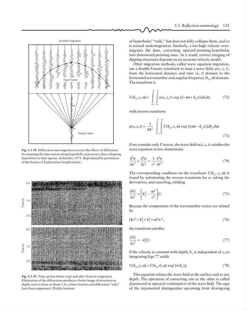
Fig. 3.3-38 Diffraction sum migration reverses the effects of diffraction
by summing the time section along hyperbolic trajectories, thus collapsing
hyperbolas to their apexes. (Schneider, 1971. Reproduced by permission
of the Society of Exploration Geophysicists.)
Time (s)
0.0
1.0
2.0
2.0
1.0
0.0
Time (s)
Fig. 3.3-39 Time section before (top) and after (bottom) migration.
Elimination of the diffractions produces a better image of structures at
depth, such as those at about 1.8 s, where bowties and diffraction “tails”
have been suppressed. (Prakla-Seismos)
Kirchoff migration
Input traces
Output trace
is termed undermigration. Similarly, a too-high velocity overmigrates the data, converting upward-pointing hyperbolas
into downward-pointing ones. As a result, correct imaging of
dipping structures depends on an accurate velocity model.
Other migration methods, called wave equation migration,
use a double Fourier transform to map a wave field, u(x, z, t),
from the horizontal distance and time (x, t) domain to the
horizontal wavenumber and angular frequency (k x , ω) domain.
The transform is
U(k x , z, ω) =
Ύ Ύ
−∞
∞
−∞
∞
u(x, z, t) exp [i(−ωt + k x x)]dxdt,
(72)
with inverse transform
u(x, z, t) =
1
4
2
π Ύ Ύ
−∞
∞
−∞
∞
U(k x , z, ω) exp [i(ωt − k x x)]dk x dω.
(73)
If we consider only P waves, the wave field u(x, z, t) satisfies the
wave equation in two dimensions:
∂
∂
∂
∂
∂
∂
2
2
2
2
2
2
2
1
u
x
u
z
v
u
t
.
+
=
(74)
The corresponding condition on the transform U(k x , z, ω) is
found by substituting the inverse transform for u, taking the
derivatives, and canceling, yielding
∂
∂
2
2
2
2
2
U
z
k
v
U
x
.
=
−
⎛
⎝
⎜
⎞
⎠
⎟
ω
(75)
Because the components of the wavenumber vector are related
by
| k | 2 = k 2
x + k 2
z = ω 2 /v 2 ,
(76)
the transform satisfies
∂
∂
2
2
2
U
z
k U
z .
= −
(77)
If the velocity is constant with depth, k z is independent of z, so
integrating Eqn 77 yields
U(k x , z, ω) = U(k x , 0, ω) exp [±ik z z].
(78)
This equation relates the wave field at the surface and at any
depth. The operation of converting one to the other is called
downward or upward continuation of the wave field. The sign
of the exponential distinguishes upcoming from downgoing
3.3 Reflection seismology 155
Fig. 3.3-38 Diffraction sum migration reverses the effects of diffraction
by summing the time section along hyperbolic trajectories, thus collapsing
hyperbolas to their apexes. (Schneider, 1971. Reproduced by permission
of the Society of Exploration Geophysicists.)
Time (s)
0.0
1.0
2.0
2.0
1.0
0.0
Time (s)
Fig. 3.3-39 Time section before (top) and after (bottom) migration.
Elimination of the diffractions produces a better image of structures at
depth, such as those at about 1.8 s, where bowties and diffraction “tails”
have been suppressed. (Prakla-Seismos)
Kirchoff migration
Input traces
Output trace