

150 Seismology and Earth Structure
Depth
Geological
section
Reflector
series
Input
pulse
Seismic
trace
*
Time
=
because the Fourier transform of a convolution equals the
product of the Fourier transforms,
S(ω) = W(ω)R(ω).
(63)
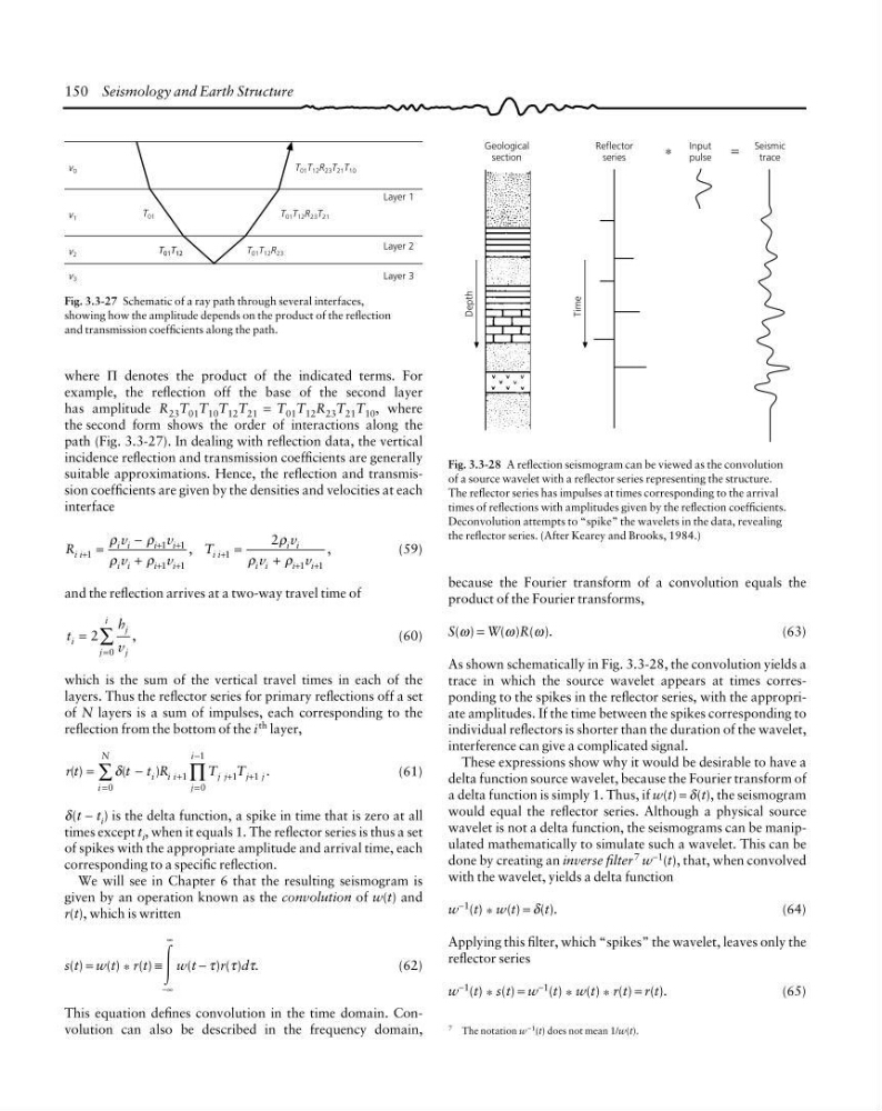
As shown schematically in Fig. 3.3-28, the convolution yields a
trace in which the source wavelet appears at times corresponding to the spikes in the reflector series, with the appropriate amplitudes. If the time between the spikes corresponding to
individual reflectors is shorter than the duration of the wavelet,
interference can give a complicated signal.
These expressions show why it would be desirable to have a
delta function source wavelet, because the Fourier transform of
a delta function is simply 1. Thus, if w(t) = δ(t), the seismogram
would equal the reflector series. Although a physical source
wavelet is not a delta function, the seismograms can be manipulated mathematically to simulate such a wavelet. This can be
done by creating an inverse filter 7 w −1 (t), that, when convolved
with the wavelet, yields a delta function
w −1 (t) * w(t) = δ(t).
(64)
Applying this filter, which “spikes” the wavelet, leaves only the
reflector series
w
−1 (t) * s(t) = w
−1 (t) * w(t) * r(t) = r(t).
(65)
Layer 1
Layer 2
Layer 3
T 01 T 12 R 23 T 21 T 10
T 01 T 12 R 23 T 21
T 01 T 12 R 23
T 01 T 12
T 01 T 12
T 01
v 0
v 1
v 2
v 3
Fig. 3.3-27 Schematic of a ray path through several interfaces,
showing how the amplitude depends on the product of the reflection
and transmission coefficients along the path.
Fig. 3.3-28 A reflection seismogram can be viewed as the convolution
of a source wavelet with a reflector series representing the structure.
The reflector series has impulses at times corresponding to the arrival
times of reflections with amplitudes given by the reflection coefficients.
Deconvolution attempts to “spike” the wavelets in the data, revealing
the reflector series. (After Kearey and Brooks, 1984.)
7 The notation w −1 (t) does not mean 1/w(t).
where Π denotes the product of the indicated terms. For
example, the reflection off the base of the second layer
has amplitude R 23 T 01 T 10 T 12 T 21 = T 01 T 12 R 23 T 21 T 10 , where
the second form shows the order of interactions along the
path (Fig. 3.3-27). In dealing with reflection data, the vertical
incidence reflection and transmission coefficients are generally
suitable approximations. Hence, the reflection and transmission coefficients are given by the densities and velocities at each
interface
R
v
v
v
v
T
v
v
v
i i
i i
i
i
i i
i
i
i i
i i
i i
i
i
,
,
+
+ +
+ +
+
+ +
=
−
+
=
+
1
1 1
1 1
1
1 1
2
ρ
ρ
ρ
ρ
ρ
ρ
ρ
(59)
and the reflection arrives at a two-way travel time of
t
h
v
i
j
j
j
i
=
=
∑ ,
2
0
(60)
which is the sum of the vertical travel times in each of the
layers. Thus the reflector series for primary reflections off a set
of N layers is a sum of impulses, each corresponding to the
reflection from the bottom of the i th layer,
r t
t t R
T T
i i i
i
N
j j
j j
j
i
( )
(
)
.
=
−
+
=
+
+
=
−
∑
∏
δ
1
0
1
1
0
1
(61)
δ(t − t i ) is the delta function, a spike in time that is zero at all
times except t i , when it equals 1. The reflector series is thus a set
of spikes with the appropriate amplitude and arrival time, each
corresponding to a specific reflection.
We will see in Chapter 6 that the resulting seismogram is
given by an operation known as the convolution of w(t) and
r(t), which is written
s(t) = w(t) * r(t) ≡ Ύ
−∞
∞
w(t − τ)r(τ)dτ.
(62)
This equation defines convolution in the time domain. Convolution can also be described in the frequency domain,
Depth
Geological
section
Reflector
series
Input
pulse
Seismic
trace
*
Time
=
because the Fourier transform of a convolution equals the
product of the Fourier transforms,
S(ω) = W(ω)R(ω).
(63)
As shown schematically in Fig. 3.3-28, the convolution yields a
trace in which the source wavelet appears at times corresponding to the spikes in the reflector series, with the appropriate amplitudes. If the time between the spikes corresponding to
individual reflectors is shorter than the duration of the wavelet,
interference can give a complicated signal.
These expressions show why it would be desirable to have a
delta function source wavelet, because the Fourier transform of
a delta function is simply 1. Thus, if w(t) = δ(t), the seismogram
would equal the reflector series. Although a physical source
wavelet is not a delta function, the seismograms can be manipulated mathematically to simulate such a wavelet. This can be
done by creating an inverse filter 7 w −1 (t), that, when convolved
with the wavelet, yields a delta function
w −1 (t) * w(t) = δ(t).
(64)
Applying this filter, which “spikes” the wavelet, leaves only the
reflector series
w
−1 (t) * s(t) = w
−1 (t) * w(t) * r(t) = r(t).
(65)
Layer 1
Layer 2
Layer 3
T 01 T 12 R 23 T 21 T 10
T 01 T 12 R 23 T 21
T 01 T 12 R 23
T 01 T 12
T 01 T 12
T 01
v 0
v 1
v 2
v 3
Fig. 3.3-27 Schematic of a ray path through several interfaces,
showing how the amplitude depends on the product of the reflection
and transmission coefficients along the path.
Fig. 3.3-28 A reflection seismogram can be viewed as the convolution
of a source wavelet with a reflector series representing the structure.
The reflector series has impulses at times corresponding to the arrival
times of reflections with amplitudes given by the reflection coefficients.
Deconvolution attempts to “spike” the wavelets in the data, revealing
the reflector series. (After Kearey and Brooks, 1984.)
7 The notation w −1 (t) does not mean 1/w(t).
where Π denotes the product of the indicated terms. For
example, the reflection off the base of the second layer
has amplitude R 23 T 01 T 10 T 12 T 21 = T 01 T 12 R 23 T 21 T 10 , where
the second form shows the order of interactions along the
path (Fig. 3.3-27). In dealing with reflection data, the vertical
incidence reflection and transmission coefficients are generally
suitable approximations. Hence, the reflection and transmission coefficients are given by the densities and velocities at each
interface
R
v
v
v
v
T
v
v
v
i i
i i
i
i
i i
i
i
i i
i i
i i
i
i
,
,
+
+ +
+ +
+
+ +
=
−
+
=
+
1
1 1
1 1
1
1 1
2
ρ
ρ
ρ
ρ
ρ
ρ
ρ
(59)
and the reflection arrives at a two-way travel time of
t
h
v
i
j
j
j
i
=
=
∑ ,
2
0
(60)
which is the sum of the vertical travel times in each of the
layers. Thus the reflector series for primary reflections off a set
of N layers is a sum of impulses, each corresponding to the
reflection from the bottom of the i th layer,
r t
t t R
T T
i i i
i
N
j j
j j
j
i
( )
(
)
.
=
−
+
=
+
+
=
−
∑
∏
δ
1
0
1
1
0
1
(61)
δ(t − t i ) is the delta function, a spike in time that is zero at all
times except t i , when it equals 1. The reflector series is thus a set
of spikes with the appropriate amplitude and arrival time, each
corresponding to a specific reflection.
We will see in Chapter 6 that the resulting seismogram is
given by an operation known as the convolution of w(t) and
r(t), which is written
s(t) = w(t) * r(t) ≡ Ύ
−∞
∞
w(t − τ)r(τ)dτ.
(62)
This equation defines convolution in the time domain. Convolution can also be described in the frequency domain,