

p 2
p 1
p 2
p 1
x
t
p 2
p 1
p
τ
2
τ
1
τ
1
τ
2
τ
3.3 Reflection seismology 147
5 Claerbout (1985).
the data, which are then transformed back to (x, t). Velocity
filters are also called dip filters, because they separate arrivals
based on their slope (dip) in the (k x , ω) domain. A variant
of this method for data recorded in two spatial dimensions,
u(x, y, t), is to take the triple Fourier transform U(k x , k y , ω).
Because the transform is in terms of both components of the
horizontal wave vector, it can be filtered to suppress arrivals
coming from certain directions.
Another approach to transforming data such that components are more easily separated uses the intercept-slowness
formulation of travel time curves. As discussed in Section 3.3.2,
the function τ(p) describes each point on a travel time curve
T(x) by the time axis intercept τ and the slope p of the line
tangential to the curve at that point. Thus seismic data can be
described as functions either of position and time, u(x, t), or of
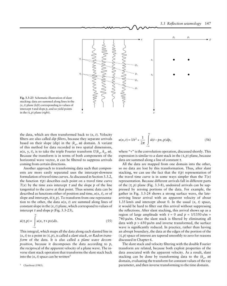
slope and intercept, I(τ, p). To transform from one representation to the other, the data u(x, t) are summed along lines of
constant slope in the (x, t) plane, which correspond to values of
intercept τ and slope p (Fig. 3.3-23),
I(τ, p) =
Ύ
−∞
∞
u(x, τ + px)dx.
(55)
This integral, which maps all the data along each slanted line in
(x, t) to a point in (τ, p), is called a slant stack, or Radon transform of the data. It is also called a plane wave decomposition, because it decomposes the data according to p,
the reciprocal of the apparent velocity of a plane wave. The inverse slant stack operation that transforms the slant stack back
into the (x, t) space can be written 5
u(x, t) = 1/t
2 *
1
2π Ύ
−∞
∞
I(t − px, p)dp,
(56)
where “ * ” is the convolution operation, discussed shortly. This
expression is similar to a slant stack in the (τ, p) plane, because
data are summed along a line of constant τ.
All the data are mapped from one domain into the other,
so no data are lost by this transformation. Thus, after slant
stacking, we can use the fact that the τ(p) representation of
the travel time curve is in some ways simpler than the T(x)
representation. Because different arrivals fall in different parts
of the (τ, p) plane (Fig. 3.3-8), undesired arrivals can be suppressed by zeroing portions of the data. For example, the
gather in Fig. 3.3-24 shows a strong surface wave, the latearriving linear arrival with an apparent velocity of about
1.35 km/s and intercept about 0. In the usual (x, t) space,
it would be hard to filter out this arrival without suppressing
the reflections. After slant stacking, this arrival shows up as a
region of large amplitude with τ ≈ 0 and p = 1/1350 s/m ≈
740 µs/m. Once the slant stack is filtered by eliminating all
data with p > 650 µs/m and inverse transformed, the surface
wave is significantly reduced. In practice, rather than having
an abrupt boundary, the data at the edges of the portion of the
(τ, p) space of interest are tapered smoothly to zero for reasons
discussed in Chapter 6.
The slant stack and velocity filtering with the double Fourier
transform are related, because both exploit properties of the
data associated with the apparent velocity. As a result, slant
stacking can be done by transforming data to the (k x , ω)
domain, evaluating the transform for constant values of the ray
parameter, and then inverse transforming to the time domain.
Fig. 3.3-23 Schematic illustration of slant
stacking: data are summed along lines in the
(x, t) plane (left) corresponding to values of
intercept τ and slope p, and so yield points
in the (τ, p) plane (right).
p 1
p 2
p 1
x
t
p 2
p 1
p
τ
2
τ
1
τ
1
τ
2
τ
3.3 Reflection seismology 147
5 Claerbout (1985).
the data, which are then transformed back to (x, t). Velocity
filters are also called dip filters, because they separate arrivals
based on their slope (dip) in the (k x , ω) domain. A variant
of this method for data recorded in two spatial dimensions,
u(x, y, t), is to take the triple Fourier transform U(k x , k y , ω).
Because the transform is in terms of both components of the
horizontal wave vector, it can be filtered to suppress arrivals
coming from certain directions.
Another approach to transforming data such that components are more easily separated uses the intercept-slowness
formulation of travel time curves. As discussed in Section 3.3.2,
the function τ(p) describes each point on a travel time curve
T(x) by the time axis intercept τ and the slope p of the line
tangential to the curve at that point. Thus seismic data can be
described as functions either of position and time, u(x, t), or of
slope and intercept, I(τ, p). To transform from one representation to the other, the data u(x, t) are summed along lines of
constant slope in the (x, t) plane, which correspond to values of
intercept τ and slope p (Fig. 3.3-23),
I(τ, p) =
Ύ
−∞
∞
u(x, τ + px)dx.
(55)
This integral, which maps all the data along each slanted line in
(x, t) to a point in (τ, p), is called a slant stack, or Radon transform of the data. It is also called a plane wave decomposition, because it decomposes the data according to p,
the reciprocal of the apparent velocity of a plane wave. The inverse slant stack operation that transforms the slant stack back
into the (x, t) space can be written 5
u(x, t) = 1/t
2 *
1
2π Ύ
−∞
∞
I(t − px, p)dp,
(56)
where “ * ” is the convolution operation, discussed shortly. This
expression is similar to a slant stack in the (τ, p) plane, because
data are summed along a line of constant τ.
All the data are mapped from one domain into the other,
so no data are lost by this transformation. Thus, after slant
stacking, we can use the fact that the τ(p) representation of
the travel time curve is in some ways simpler than the T(x)
representation. Because different arrivals fall in different parts
of the (τ, p) plane (Fig. 3.3-8), undesired arrivals can be suppressed by zeroing portions of the data. For example, the
gather in Fig. 3.3-24 shows a strong surface wave, the latearriving linear arrival with an apparent velocity of about
1.35 km/s and intercept about 0. In the usual (x, t) space,
it would be hard to filter out this arrival without suppressing
the reflections. After slant stacking, this arrival shows up as a
region of large amplitude with τ ≈ 0 and p = 1/1350 s/m ≈
740 µs/m. Once the slant stack is filtered by eliminating all
data with p > 650 µs/m and inverse transformed, the surface
wave is significantly reduced. In practice, rather than having
an abrupt boundary, the data at the edges of the portion of the
(τ, p) space of interest are tapered smoothly to zero for reasons
discussed in Chapter 6.
The slant stack and velocity filtering with the double Fourier
transform are related, because both exploit properties of the
data associated with the apparent velocity. As a result, slant
stacking can be done by transforming data to the (k x , ω)
domain, evaluating the transform for constant values of the ray
parameter, and then inverse transforming to the time domain.
Fig. 3.3-23 Schematic illustration of slant
stacking: data are summed along lines in the
(x, t) plane (left) corresponding to values of
intercept τ and slope p, and so yield points
in the (τ, p) plane (right).