

146 Seismology and Earth Structure
0.0
0.1
0.2
0.3
0.4
0.5
0.6
0.7
0.8
0.9
1.0
1.1
1.2
1.3
1.4
1.5
1.6
1.7
1.8
1.9
2.0
0.0
0.1
0.2
0.3
0.4
0.5
0.6
0.7
0.8
0.9
1.0
1.1
1.2
1.3
1.4
1.5
1.6
1.7
1.8
1.9
2.0
0.0
0.1
0.2
0.3
0.4
0.5
0.6
0.7
0.8
0.9
1.0
1.1
1.2
1.3
1.4
1.5
1.6
1.7
1.8
1.9
2.0
0.0
0.1
0.2
0.3
0.4
0.5
0.6
0.7
0.8
0.9
1.0
1.1
1.2
1.3
1.4
1.5
1.6
1.7
1.8
1.9
2.0
Raw shot record
Shot record with f–k filter
120
100
80
60
40
20
0
∞
−0.002
−500
−0.004
−250
0.004
250
0.002
500
k (1/ft)
λ (ft)
1 0 ,0 0 0 f t /s
3 0 ,0 0 0 f t /s
60 ,0 00 ft /s
Side
wind
noise
Scattered
near-surface
noise
Surface waves
Air waves
Reflected signals
Frequency (Hz)
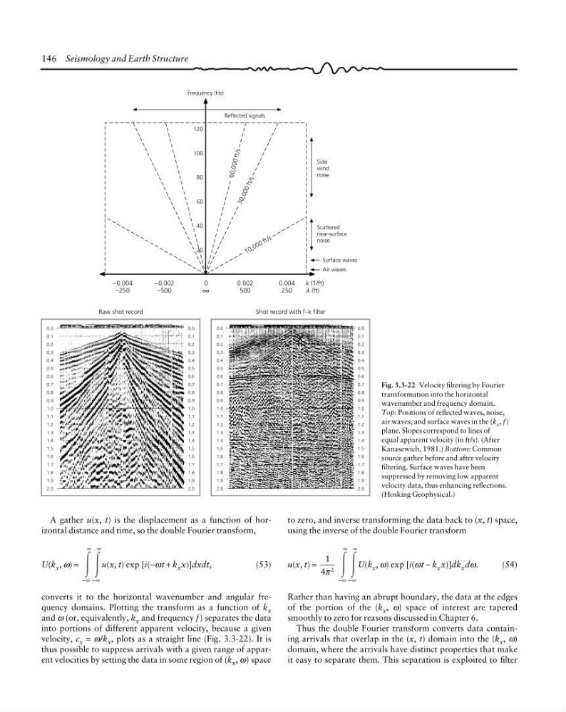
Fig. 3.3-22 Velocity filtering by Fourier
transformation into the horizontal
wavenumber and frequency domain.
Top: Positions of reflected waves, noise,
air waves, and surface waves in the (k x , f )
plane. Slopes correspond to lines of
equal apparent velocity (in ft/s). (After
Kanasewich, 1981.) Bottom: Common
source gather before and after velocity
filtering. Surface waves have been
suppressed by removing low apparent
velocity data, thus enhancing reflections.
(Hosking Geophysical.)
A gather u(x, t) is the displacement as a function of horizontal distance and time, so the double Fourier transform,
U(k x , ω) =
Ύ Ύ
−∞
∞
−∞
∞
u(x, t) exp [i(−ωt + k x x)]dxdt,
(53)
converts it to the horizontal wavenumber and angular frequency domains. Plotting the transform as a function of k x
and ω (or, equivalently, k x and frequency f ) separates the data
into portions of different apparent velocity, because a given
velocity, c x = ω/k x , plots as a straight line (Fig. 3.3-22). It is
thus possible to suppress arrivals with a given range of apparent velocities by setting the data in some region of (k x , ω) space
to zero, and inverse transforming the data back to (x, t) space,
using the inverse of the double Fourier transform
u(x, t) =
1
4
2
π Ύ Ύ
−∞
∞
−∞
∞
U(k x , ω) exp [i(ωt − k x x)]dk x dω.
(54)
Rather than having an abrupt boundary, the data at the edges
of the portion of the (k x , ω) space of interest are tapered
smoothly to zero for reasons discussed in Chapter 6.
Thus the double Fourier transform converts data containing arrivals that overlap in the (x, t) domain into the (k x , ω)
domain, where the arrivals have distinct properties that make
it easy to separate them. This separation is exploited to filter
0.0
0.1
0.2
0.3
0.4
0.5
0.6
0.7
0.8
0.9
1.0
1.1
1.2
1.3
1.4
1.5
1.6
1.7
1.8
1.9
2.0
0.0
0.1
0.2
0.3
0.4
0.5
0.6
0.7
0.8
0.9
1.0
1.1
1.2
1.3
1.4
1.5
1.6
1.7
1.8
1.9
2.0
0.0
0.1
0.2
0.3
0.4
0.5
0.6
0.7
0.8
0.9
1.0
1.1
1.2
1.3
1.4
1.5
1.6
1.7
1.8
1.9
2.0
0.0
0.1
0.2
0.3
0.4
0.5
0.6
0.7
0.8
0.9
1.0
1.1
1.2
1.3
1.4
1.5
1.6
1.7
1.8
1.9
2.0
Raw shot record
Shot record with f–k filter
120
100
80
60
40
20
0
∞
−0.002
−500
−0.004
−250
0.004
250
0.002
500
k (1/ft)
λ (ft)
1 0 ,0 0 0 f t /s
3 0 ,0 0 0 f t /s
60 ,0 00 ft /s
Side
wind
noise
Scattered
near-surface
noise
Surface waves
Air waves
Reflected signals
Frequency (Hz)
Fig. 3.3-22 Velocity filtering by Fourier
transformation into the horizontal
wavenumber and frequency domain.
Top: Positions of reflected waves, noise,
air waves, and surface waves in the (k x , f )
plane. Slopes correspond to lines of
equal apparent velocity (in ft/s). (After
Kanasewich, 1981.) Bottom: Common
source gather before and after velocity
filtering. Surface waves have been
suppressed by removing low apparent
velocity data, thus enhancing reflections.
(Hosking Geophysical.)
A gather u(x, t) is the displacement as a function of horizontal distance and time, so the double Fourier transform,
U(k x , ω) =
Ύ Ύ
−∞
∞
−∞
∞
u(x, t) exp [i(−ωt + k x x)]dxdt,
(53)
converts it to the horizontal wavenumber and angular frequency domains. Plotting the transform as a function of k x
and ω (or, equivalently, k x and frequency f ) separates the data
into portions of different apparent velocity, because a given
velocity, c x = ω/k x , plots as a straight line (Fig. 3.3-22). It is
thus possible to suppress arrivals with a given range of apparent velocities by setting the data in some region of (k x , ω) space
to zero, and inverse transforming the data back to (x, t) space,
using the inverse of the double Fourier transform
u(x, t) =
1
4
2
π Ύ Ύ
−∞
∞
−∞
∞
U(k x , ω) exp [i(ωt − k x x)]dk x dω.
(54)
Rather than having an abrupt boundary, the data at the edges
of the portion of the (k x , ω) space of interest are tapered
smoothly to zero for reasons discussed in Chapter 6.
Thus the double Fourier transform converts data containing arrivals that overlap in the (x, t) domain into the (k x , ω)
domain, where the arrivals have distinct properties that make
it easy to separate them. This separation is exploited to filter