

B
C
D
H a lf -o ff s e t h
H a lf -o ff se t h
H a lf -o ff se t h
H a lf -o ff s e t h
m 1
m 2
m 3
m 4
midpoint, m
F
E
D′
E′
C′
B′
A
Time,
t
3.3 Reflection seismology 143
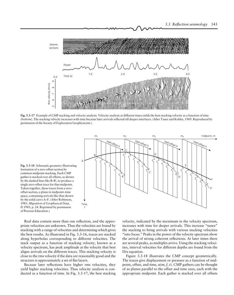
Fig. 3.3-17 Example of CMP stacking and velocity analysis. Velocity analysis at different times yields the best stacking velocity as a function of time
(bottom). The stacking velocity increases with time because later arrivals reflected off deeper interfaces. (After Taner and Kohler, 1969. Reproduced by
permission of the Society of Exploration Geophysicists.)
Rms velocity (km /s)
5
Seismic
sections
Power
Time (s)
1.0
2.0
3.0
4.0
6
7
8
9
0.0
Real data contain more than one reflection, and the appropriate velocities are unknown. Thus the velocities are found by
stacking with a range of velocities and determining which gives
the best results. As illustrated in Fig. 3.3-16, traces are stacked
along hyperbolas corresponding to different velocities. The
stack output as a function of stacking velocity, known as a
velocity spectrum, has peak amplitude at the velocity that best
aligns arrivals on the different traces. This stacking velocity is
close to the rms velocity if the data are reasonably good and the
structure is approximately a set of flat layers.
Because later reflections have higher rms velocities, they
yield higher stacking velocities. Thus velocity analysis is conducted as a function of time. In Fig. 3.3-17, the best stacking
velocity, indicated by the maximum in the velocity spectrum,
increases with time for deeper arrivals. This increase “tunes”
the stacking to bring arrivals with various stacking velocities
“into focus.” Peaks in the power of the velocity spectrum show
the arrival of strong coherent reflections. At later times there
are several peaks, as multiples arrive. Using the stacking velocities, interval velocities for different depths are found from the
Dix equation.
Figure 3.3-18 illustrates the CMP concept geometrically.
The traces give displacement or pressure as a function of midpoint, offset, and time, u(m, f, t). CMP gathers can be thought
of as planes parallel to the offset and time axes, each with the
appropriate midpoint. Each gather is stacked over all offsets
Fig. 3.3-18 Schematic geometry illustrating
formation of a zero-offset section by
common midpoint stacking. Each CMP
gather is stacked over all offsets, as shown
by the dashed lines like B–B′, to produce a
single zero-offset trace for that midpoint.
Taken together, these traces form a zerooffset section, a plane in midpoint–time
space, containing arrivals like that shown
by the solid curve A–F. (After Robinson,
1983. Migration of Geophysical Data,
© 1983, p. 24. Reprinted by permission
of Pearson Education.)
C
D
H a lf -o ff s e t h
H a lf -o ff se t h
H a lf -o ff se t h
H a lf -o ff s e t h
m 1
m 2
m 3
m 4
midpoint, m
F
E
D′
E′
C′
B′
A
Time,
t
3.3 Reflection seismology 143
Fig. 3.3-17 Example of CMP stacking and velocity analysis. Velocity analysis at different times yields the best stacking velocity as a function of time
(bottom). The stacking velocity increases with time because later arrivals reflected off deeper interfaces. (After Taner and Kohler, 1969. Reproduced by
permission of the Society of Exploration Geophysicists.)
Rms velocity (km /s)
5
Seismic
sections
Power
Time (s)
1.0
2.0
3.0
4.0
6
7
8
9
0.0
Real data contain more than one reflection, and the appropriate velocities are unknown. Thus the velocities are found by
stacking with a range of velocities and determining which gives
the best results. As illustrated in Fig. 3.3-16, traces are stacked
along hyperbolas corresponding to different velocities. The
stack output as a function of stacking velocity, known as a
velocity spectrum, has peak amplitude at the velocity that best
aligns arrivals on the different traces. This stacking velocity is
close to the rms velocity if the data are reasonably good and the
structure is approximately a set of flat layers.
Because later reflections have higher rms velocities, they
yield higher stacking velocities. Thus velocity analysis is conducted as a function of time. In Fig. 3.3-17, the best stacking
velocity, indicated by the maximum in the velocity spectrum,
increases with time for deeper arrivals. This increase “tunes”
the stacking to bring arrivals with various stacking velocities
“into focus.” Peaks in the power of the velocity spectrum show
the arrival of strong coherent reflections. At later times there
are several peaks, as multiples arrive. Using the stacking velocities, interval velocities for different depths are found from the
Dix equation.
Figure 3.3-18 illustrates the CMP concept geometrically.
The traces give displacement or pressure as a function of midpoint, offset, and time, u(m, f, t). CMP gathers can be thought
of as planes parallel to the offset and time axes, each with the
appropriate midpoint. Each gather is stacked over all offsets
Fig. 3.3-18 Schematic geometry illustrating
formation of a zero-offset section by
common midpoint stacking. Each CMP
gather is stacked over all offsets, as shown
by the dashed lines like B–B′, to produce a
single zero-offset trace for that midpoint.
Taken together, these traces form a zerooffset section, a plane in midpoint–time
space, containing arrivals like that shown
by the solid curve A–F. (After Robinson,
1983. Migration of Geophysical Data,
© 1983, p. 24. Reprinted by permission
of Pearson Education.)