

138 Seismology and Earth Structure
τ(p) = T(p) − px(p),
(38)
and differentiate
d
dp
dT
dp
p
dx
dp
x p
dT
dx
dx
dp
p
dx
dp
x p
x p
τ
( )
( )
( ).
=
−
−
=
−
−
= −
(39)
Thus, just as p is the slope of the travel time curve, T(x), the
distance, x, is minus the slope of the τ(p) curve.
To illustrate these ideas, we show that the τ(p) formulation
gives the travel time curve for the reflected wave in a layer over
a halfspace. Figure 3.3-3 shows that x 0 = x/2, so, using Eqn 32,
p
x
v x
h
h
v x
h
( / )
[( / )
]
,
[( / )
]
.
/
/
=
+
=
+
2
2
2
0
2
0
2 1 2
0
0
0
2
0
2 1 2
η
(40)
Hence, by Eqns 36 and 37, the travel time curve is
T(x) = px + 2η 0 h 0 =
( / )
[( / )
] /
x
h
v x
h
2
0
2
0
2
0
2 1 2
2 2
2
+
+
= 2[(x/2)
2
+ h
2
0 ]
1/2
/v 0 ,
(41)
which is the familiar hyperbola (Eqn 9).
To see how this travel time curve appears when written as
τ(p), we write Eqn 37 for a layer over a halfspace:
τ(p) = 2(1/v 2
0 − p 2 ) 1/2 h 0 .
(42)
This can also be written as
(v
2
0 τ 2 )/(4h 2
0 ) + v 2
0 p 2 = 1,
(43)
which is an ellipse whose axes are the τ and p axes (Fig. 3.3-8).
It intersects the τ axis at (τ = t 0 = 2h 0 /v 0 , p = 0), and the p axis at
(τ = 0, p = 1/v 0 ). Both these points have significance. The first,
where the travel time curve has zero slope and the time axis
intercept is the vertical two-way travel time, corresponds to
the zero-offset point x = 0.
The second, where the travel time curve has slope 1/v 0 and
time axis intercept 0, is the τ(p) position of the linear travel
time curve for the direct wave. Hence the line for the direct
wave maps to a point in the τ(p) plane that is on the ellipse
describing the reflected wave. To understand why this occurs,
we use the fact that distance is minus the derivative of the τ(p)
curve (Eqn 39) and differentiate Eqn 42, giving
x(p) = −dτ /dp = 2ph 0 (1/v 2
0 − p 2 ) −1/2 ,
(44)
so at the point p = 1/v 0 , x = ∞. This makes sense, because as
x → ∞, the reflected wave is asymptotic to the direct wave
(Fig. 3.2-2).
The head wave is easily mapped into the τ (p) plane, because
its travel time curve (Eqn 3.2.8) is
T x
T
p x
h
j
j
n
j j
j
n
j j
j
n
( )
.
=
=
+
=
=
=
∑
∑
∑
2
2
2
0
0
0
∆
η
(34)
By Snell’s law, the horizontal ray parameter is constant along
the ray path, so p j = p, and
T x px
h
j j
j
n
( )
,
=
+
=
∑
2
0
η
(35)
where x = 2 ∑
=
j
n
0
x j is the total horizontal distance traveled. This
formulation is equivalent to the way we formulated the travel
time as the scalar product of the distance and slowness vectors
(Eqn 2.5.34).
Formulating the travel time curve in this way gives interesting insight. We define
T(x) = px + τ(p),
(36)
where the function
τ
η
( )
( /
)
(
)
.
/
/
p
h
v
p
h
u
p
h
j j
j
n
j
j
j
n
j
j
j
n
=
=
−
=
−
=
=
=
∑
∑
∑
2
2
1
2
0
2
212
0
2
212
0
(37)
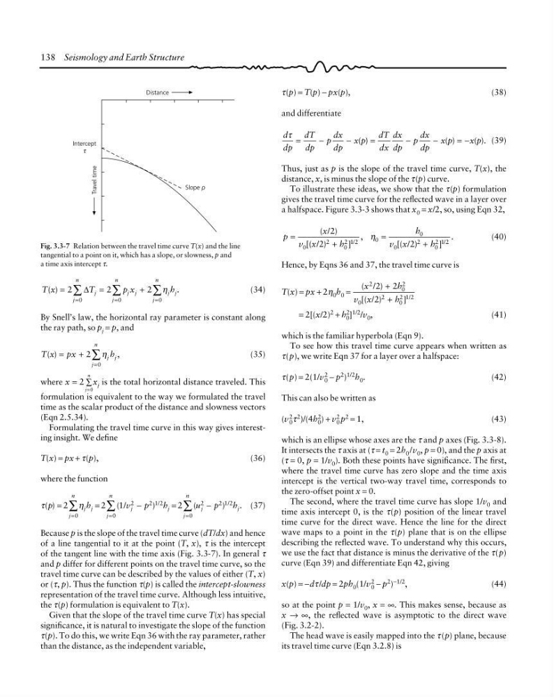
Because p is the slope of the travel time curve (dT/dx) and hence
of a line tangential to it at the point (T, x), τ is the intercept
of the tangent line with the time axis (Fig. 3.3-7). In general τ
and p differ for different points on the travel time curve, so the
travel time curve can be described by the values of either (T, x)
or (τ, p). Thus the function τ(p) is called the intercept-slowness
representation of the travel time curve. Although less intuitive,
the τ(p) formulation is equivalent to T(x).
Given that the slope of the travel time curve T(x) has special
significance, it is natural to investigate the slope of the function
τ(p). To do this, we write Eqn 36 with the ray parameter, rather
than the distance, as the independent variable,
Fig. 3.3-7 Relation between the travel time curve T(x) and the line
tangential to a point on it, which has a slope, or slowness, p and
a time axis intercept τ.
Distance
Slope p
Travel time
Intercept
τ
τ(p) = T(p) − px(p),
(38)
and differentiate
d
dp
dT
dp
p
dx
dp
x p
dT
dx
dx
dp
p
dx
dp
x p
x p
τ
( )
( )
( ).
=
−
−
=
−
−
= −
(39)
Thus, just as p is the slope of the travel time curve, T(x), the
distance, x, is minus the slope of the τ(p) curve.
To illustrate these ideas, we show that the τ(p) formulation
gives the travel time curve for the reflected wave in a layer over
a halfspace. Figure 3.3-3 shows that x 0 = x/2, so, using Eqn 32,
p
x
v x
h
h
v x
h
( / )
[( / )
]
,
[( / )
]
.
/
/
=
+
=
+
2
2
2
0
2
0
2 1 2
0
0
0
2
0
2 1 2
η
(40)
Hence, by Eqns 36 and 37, the travel time curve is
T(x) = px + 2η 0 h 0 =
( / )
[( / )
] /
x
h
v x
h
2
0
2
0
2
0
2 1 2
2 2
2
+
+
= 2[(x/2)
2
+ h
2
0 ]
1/2
/v 0 ,
(41)
which is the familiar hyperbola (Eqn 9).
To see how this travel time curve appears when written as
τ(p), we write Eqn 37 for a layer over a halfspace:
τ(p) = 2(1/v 2
0 − p 2 ) 1/2 h 0 .
(42)
This can also be written as
(v
2
0 τ 2 )/(4h 2
0 ) + v 2
0 p 2 = 1,
(43)
which is an ellipse whose axes are the τ and p axes (Fig. 3.3-8).
It intersects the τ axis at (τ = t 0 = 2h 0 /v 0 , p = 0), and the p axis at
(τ = 0, p = 1/v 0 ). Both these points have significance. The first,
where the travel time curve has zero slope and the time axis
intercept is the vertical two-way travel time, corresponds to
the zero-offset point x = 0.
The second, where the travel time curve has slope 1/v 0 and
time axis intercept 0, is the τ(p) position of the linear travel
time curve for the direct wave. Hence the line for the direct
wave maps to a point in the τ(p) plane that is on the ellipse
describing the reflected wave. To understand why this occurs,
we use the fact that distance is minus the derivative of the τ(p)
curve (Eqn 39) and differentiate Eqn 42, giving
x(p) = −dτ /dp = 2ph 0 (1/v 2
0 − p 2 ) −1/2 ,
(44)
so at the point p = 1/v 0 , x = ∞. This makes sense, because as
x → ∞, the reflected wave is asymptotic to the direct wave
(Fig. 3.2-2).
The head wave is easily mapped into the τ (p) plane, because
its travel time curve (Eqn 3.2.8) is
T x
T
p x
h
j
j
n
j j
j
n
j j
j
n
( )
.
=
=
+
=
=
=
∑
∑
∑
2
2
2
0
0
0
∆
η
(34)
By Snell’s law, the horizontal ray parameter is constant along
the ray path, so p j = p, and
T x px
h
j j
j
n
( )
,
=
+
=
∑
2
0
η
(35)
where x = 2 ∑
=
j
n
0
x j is the total horizontal distance traveled. This
formulation is equivalent to the way we formulated the travel
time as the scalar product of the distance and slowness vectors
(Eqn 2.5.34).
Formulating the travel time curve in this way gives interesting insight. We define
T(x) = px + τ(p),
(36)
where the function
τ
η
( )
( /
)
(
)
.
/
/
p
h
v
p
h
u
p
h
j j
j
n
j
j
j
n
j
j
j
n
=
=
−
=
−
=
=
=
∑
∑
∑
2
2
1
2
0
2
212
0
2
212
0
(37)
Because p is the slope of the travel time curve (dT/dx) and hence
of a line tangential to it at the point (T, x), τ is the intercept
of the tangent line with the time axis (Fig. 3.3-7). In general τ
and p differ for different points on the travel time curve, so the
travel time curve can be described by the values of either (T, x)
or (τ, p). Thus the function τ(p) is called the intercept-slowness
representation of the travel time curve. Although less intuitive,
the τ(p) formulation is equivalent to T(x).
Given that the slope of the travel time curve T(x) has special
significance, it is natural to investigate the slope of the function
τ(p). To do this, we write Eqn 36 with the ray parameter, rather
than the distance, as the independent variable,
Fig. 3.3-7 Relation between the travel time curve T(x) and the line
tangential to a point on it, which has a slope, or slowness, p and
a time axis intercept τ.
Distance
Slope p
Travel time
Intercept
τ