

S
N
4
2
0
T – X /6.0 (s)
Depth (km)
Band of N–S
striking faults
0
1 0
2 0
3 0
Distance (km)
40
50
10
5
4.0
3.95
3.5
3.6
4.2
5.5
5.8
3.2 Refraction seismology 127
also fits the travel times showing several velocity increases
beyond this distance.
The restriction of uniform-velocity layers can also be surmounted. Geological instincts (a useful but occasionally unreliable tool) lead us to expect that rock types, and thus velocities,
should often vary smoothly rather than in discrete jumps. Thus
we expect velocity gradients with depth, rather than sharp interfaces. This possibility can be tested using advanced methods
of analysis that predict both the travel times and the amplitudes
of the expected arrivals. The amplitudes make it possible to
distinguish gradients from uniform layers, even if the travel
times predicted are the same. Although the methods are beyond
our scope here, we discuss some results briefly.
To illustrate the relation between velocity structure and
amplitudes, consider theoretical, or synthetic, seismogram record sections for the head wave, P n , and Moho reflection, P m P,
predicted by two crustal models (Fig. 3.2-14). The seismograms were computed using a method known as reflectivity,
which avoids the limitations of ray and plane wave analysis.
The travel times are reduced at 8 km/s, and the direct wave
is not shown. Both models have the same average velocity
structure, a 30 km-thick layer of 6.5 km/s material over an
8 km/s halfspace, so the travel times are similar. However, the
amplitudes of the arrivals differ noticeably because the models
have different fine structure near the Moho.
For the sharp Moho model (Fig. 3.2-14, top) the reflected
wave is small for distances less than the critical distance
(subcritical reflection), largest near the critical distance, and
large for distances greater than critical (supercritical, postcritical, or wide angle reflections). Because the boundary is sharp,
this amplitude behavior is similar to that predicted for plane
waves (Fig. 2.6-11). P m P also shows the expected phase shift
for reflection past critical incidence (Section 2.6.4). The head
wave first appears near the critical distance, 83 km, and is
small, as expected from the plane wave approximation that
predicts no transmitted wave past the critical angle.
Figure 3.2-14 (bottom) shows the effect of velocity gradients
above and below the Moho. Seismic energy trapped near the
Moho yields larger P n amplitudes than for the sharp Moho
case. In addition, for subcritical distances, the reflection is
smaller than without a gradient above the Moho, because it
no longer reflects off a sharp interface. Hence the amplitudes
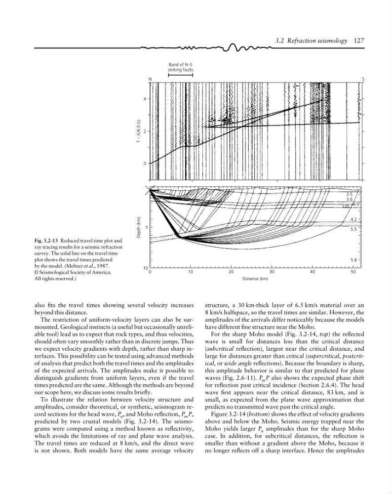
Fig. 3.2-13 Reduced travel time plot and
ray tracing results for a seismic refraction
survey. The solid line on the travel time
plot shows the travel times predicted
by the model. (Meltzer et al., 1987.
© Seismological Society of America.
All rights reserved.)
N
4
2
0
T – X /6.0 (s)
Depth (km)
Band of N–S
striking faults
0
1 0
2 0
3 0
Distance (km)
40
50
10
5
4.0
3.95
3.5
3.6
4.2
5.5
5.8
3.2 Refraction seismology 127
also fits the travel times showing several velocity increases
beyond this distance.
The restriction of uniform-velocity layers can also be surmounted. Geological instincts (a useful but occasionally unreliable tool) lead us to expect that rock types, and thus velocities,
should often vary smoothly rather than in discrete jumps. Thus
we expect velocity gradients with depth, rather than sharp interfaces. This possibility can be tested using advanced methods
of analysis that predict both the travel times and the amplitudes
of the expected arrivals. The amplitudes make it possible to
distinguish gradients from uniform layers, even if the travel
times predicted are the same. Although the methods are beyond
our scope here, we discuss some results briefly.
To illustrate the relation between velocity structure and
amplitudes, consider theoretical, or synthetic, seismogram record sections for the head wave, P n , and Moho reflection, P m P,
predicted by two crustal models (Fig. 3.2-14). The seismograms were computed using a method known as reflectivity,
which avoids the limitations of ray and plane wave analysis.
The travel times are reduced at 8 km/s, and the direct wave
is not shown. Both models have the same average velocity
structure, a 30 km-thick layer of 6.5 km/s material over an
8 km/s halfspace, so the travel times are similar. However, the
amplitudes of the arrivals differ noticeably because the models
have different fine structure near the Moho.
For the sharp Moho model (Fig. 3.2-14, top) the reflected
wave is small for distances less than the critical distance
(subcritical reflection), largest near the critical distance, and
large for distances greater than critical (supercritical, postcritical, or wide angle reflections). Because the boundary is sharp,
this amplitude behavior is similar to that predicted for plane
waves (Fig. 2.6-11). P m P also shows the expected phase shift
for reflection past critical incidence (Section 2.6.4). The head
wave first appears near the critical distance, 83 km, and is
small, as expected from the plane wave approximation that
predicts no transmitted wave past the critical angle.
Figure 3.2-14 (bottom) shows the effect of velocity gradients
above and below the Moho. Seismic energy trapped near the
Moho yields larger P n amplitudes than for the sharp Moho
case. In addition, for subcritical distances, the reflection is
smaller than without a gradient above the Moho, because it
no longer reflects off a sharp interface. Hence the amplitudes
Fig. 3.2-13 Reduced travel time plot and
ray tracing results for a seismic refraction
survey. The solid line on the travel time
plot shows the travel times predicted
by the model. (Meltzer et al., 1987.
© Seismological Society of America.
All rights reserved.)