

108 Basic Seismological Theory
lines of successively higher eigenfrequencies (shorter periods)
define overtone branches with increasing n. On any branch, the
eigenfrequency increases for higher angular order l.
As we have seen, the angular order l relates modes to
traveling waves of a specific wavelength (Eqn 20) or phase
velocity (Eqn 21). Thus frequency–angular order plots for
normal modes as in Fig. 2.9-10 correspond to dispersion (phase
velocity–period) plots for surface waves (Fig. 2.7-8) and are
sometimes called normal mode dispersion plots.
Various regions of the torsional mode dispersion plot in
Fig. 2.9-10 correspond to different body and surface shear wave
(SH) phases, which are discussed further in the next chapter.
The horizontal phase velocity (Eqn 21) of the waves corresponding to a given mode can be related to the horizontal
phase velocity of a surface wave or the apparent velocity of
a body wave phase. The upper left of the figure, with high
frequency and low angular order l, contains modes that contribute to body wave phases with high apparent velocities
and thus near-vertical incidence (recall from Section 2.5.3) that
c x = v/sin i), such as the core reflections (Figs 1.1-2 and 3.5-5)
ScS, sScS, and ScS 2 . The dashed line corresponds to modes with
a phase velocity around 7.3 km/s, which is the apparent velocity of shear waves that diffract around the core. We will see
that these SH diff waves bottom and turn at the core–mantle
boundary, and so represent the transition between direct S and
ScS, which reflects at the core–mantle boundary. To the right
of the dashed line are modes corresponding to S wave phases
that bottom in the mantle, like S, SS, sS, sSS, and SSS. Modes
further to the right (higher l) for a given frequency have lower
phase velocity, and thus correspond to body wave phases (Section 3.4) that bottom at shallower depths in the mantle. The
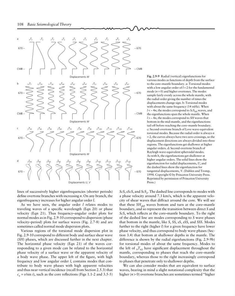
difference is shown by the radial eigenfunctions (Fig. 2.9-9b)
for torsional modes of about the same frequency. Modes to
the left of 9 T 43 have significant displacement throughout the
mantle, corresponding to phases that reach the core–mantle
boundary, whereas those to the right increasingly correspond
to phases that penetrate only to shallower depths.
We can also consider modes that are equivalent to surface
waves, bearing in mind a slight notational complexity that the
higher (n > 0) overtone branches are sometimes termed “higher
670 –
Displacements U, V
d
2 S 30
2 S 130
2 S 40
2 S 50
2 S 60
2 S 70
2 S 80
2 S 90
2 S 100
2 S 110
2 S 120
– 670
670 –
Displacements W
c
2 T 30
2 T 130
2 T 40
2 T 50
2 T 60
2 T 70
2 T 80
2 T 90
2 T 100
2 T 110
2 T 120
– 670
CMB –
Displacements W
b
13 T 7
4 T 67
12 T 25
11 T 34
10 T 40
9 T 43
8 T 47
7 T 51
6 T 55
– CMB
670 –
– 670
5 T 61
CMB –
Displacements W
a
0 T 2
9 T 2
1 T 2
2 T 2
3 T 2
4 T 2
5 T 2
6 T 2
7 T 2
– CMB
670 –
– 670
8 T 2
Fig. 2.9-9 Radial (vertical) eigenfunctions for
various modes as functions of depth from the surface
to the core–mantle boundary. a: Torsional modes
with a low angular order of l = 2 for the fundamental
mode (n = 0) and higher overtones. The modes
sample fairly evenly across the whole mantle, with
the radial order giving the number of times the
displacements change sign. b: Torsional modes
with about the same frequency (14 mHz). When
l < ~ 4n, the modes correspond to ScS SH waves, and
the eigenfunctions span the whole mantle. When
l > ~ 4n, the modes correspond to SH waves that
bottom in the mid-mantle, and the eigenfunctions
tail off before reaching the core–mantle boundary.
c: Second-overtone branch of Love wave-equivalent
torsional modes. Because the radial order is always n
= 2, the curves always have two zero crossings, so the
displacement directions are always divided into three
regions. The eigenfunctions get shallower at higher
angular orders. d: Second-overtone branch of
Rayleigh wave-equivalent spheroidal modes.
As with b, the eigenfunctions get shallower at
higher angular orders. The solid lines show the
eigenfunction for radial displacements, U, and
the dashed lines show the eigenfunction for
tangential displacements, V. (Dahlen and Tromp,
1998. Copyright © by Princeton University Press.
Reprinted by permission of Princeton University
Press.)
lines of successively higher eigenfrequencies (shorter periods)
define overtone branches with increasing n. On any branch, the
eigenfrequency increases for higher angular order l.
As we have seen, the angular order l relates modes to
traveling waves of a specific wavelength (Eqn 20) or phase
velocity (Eqn 21). Thus frequency–angular order plots for
normal modes as in Fig. 2.9-10 correspond to dispersion (phase
velocity–period) plots for surface waves (Fig. 2.7-8) and are
sometimes called normal mode dispersion plots.
Various regions of the torsional mode dispersion plot in
Fig. 2.9-10 correspond to different body and surface shear wave
(SH) phases, which are discussed further in the next chapter.
The horizontal phase velocity (Eqn 21) of the waves corresponding to a given mode can be related to the horizontal
phase velocity of a surface wave or the apparent velocity of
a body wave phase. The upper left of the figure, with high
frequency and low angular order l, contains modes that contribute to body wave phases with high apparent velocities
and thus near-vertical incidence (recall from Section 2.5.3) that
c x = v/sin i), such as the core reflections (Figs 1.1-2 and 3.5-5)
ScS, sScS, and ScS 2 . The dashed line corresponds to modes with
a phase velocity around 7.3 km/s, which is the apparent velocity of shear waves that diffract around the core. We will see
that these SH diff waves bottom and turn at the core–mantle
boundary, and so represent the transition between direct S and
ScS, which reflects at the core–mantle boundary. To the right
of the dashed line are modes corresponding to S wave phases
that bottom in the mantle, like S, SS, sS, sSS, and SSS. Modes
further to the right (higher l) for a given frequency have lower
phase velocity, and thus correspond to body wave phases (Section 3.4) that bottom at shallower depths in the mantle. The
difference is shown by the radial eigenfunctions (Fig. 2.9-9b)
for torsional modes of about the same frequency. Modes to
the left of 9 T 43 have significant displacement throughout the
mantle, corresponding to phases that reach the core–mantle
boundary, whereas those to the right increasingly correspond
to phases that penetrate only to shallower depths.
We can also consider modes that are equivalent to surface
waves, bearing in mind a slight notational complexity that the
higher (n > 0) overtone branches are sometimes termed “higher
670 –
Displacements U, V
d
2 S 30
2 S 130
2 S 40
2 S 50
2 S 60
2 S 70
2 S 80
2 S 90
2 S 100
2 S 110
2 S 120
– 670
670 –
Displacements W
c
2 T 30
2 T 130
2 T 40
2 T 50
2 T 60
2 T 70
2 T 80
2 T 90
2 T 100
2 T 110
2 T 120
– 670
CMB –
Displacements W
b
13 T 7
4 T 67
12 T 25
11 T 34
10 T 40
9 T 43
8 T 47
7 T 51
6 T 55
– CMB
670 –
– 670
5 T 61
CMB –
Displacements W
a
0 T 2
9 T 2
1 T 2
2 T 2
3 T 2
4 T 2
5 T 2
6 T 2
7 T 2
– CMB
670 –
– 670
8 T 2
Fig. 2.9-9 Radial (vertical) eigenfunctions for
various modes as functions of depth from the surface
to the core–mantle boundary. a: Torsional modes
with a low angular order of l = 2 for the fundamental
mode (n = 0) and higher overtones. The modes
sample fairly evenly across the whole mantle, with
the radial order giving the number of times the
displacements change sign. b: Torsional modes
with about the same frequency (14 mHz). When
l < ~ 4n, the modes correspond to ScS SH waves, and
the eigenfunctions span the whole mantle. When
l > ~ 4n, the modes correspond to SH waves that
bottom in the mid-mantle, and the eigenfunctions
tail off before reaching the core–mantle boundary.
c: Second-overtone branch of Love wave-equivalent
torsional modes. Because the radial order is always n
= 2, the curves always have two zero crossings, so the
displacement directions are always divided into three
regions. The eigenfunctions get shallower at higher
angular orders. d: Second-overtone branch of
Rayleigh wave-equivalent spheroidal modes.
As with b, the eigenfunctions get shallower at
higher angular orders. The solid lines show the
eigenfunction for radial displacements, U, and
the dashed lines show the eigenfunction for
tangential displacements, V. (Dahlen and Tromp,
1998. Copyright © by Princeton University Press.
Reprinted by permission of Princeton University
Press.)