

Frequency (Hz)
0.08
0.06
0.04
0.02
0
0
Angular order (l)
S diff
1000
Frequency (Hz)
0.003
0.002
0.001
0
0
Angular order (l)
0 T 2
10
200
600
800
400
2
4
6
8
0 T 3
1 T 2
1 T 1
n = 3
n = 2
n = 1
n = 0
Love
S
ScS
n = 10
n = 1
n = 0
Torsional modes
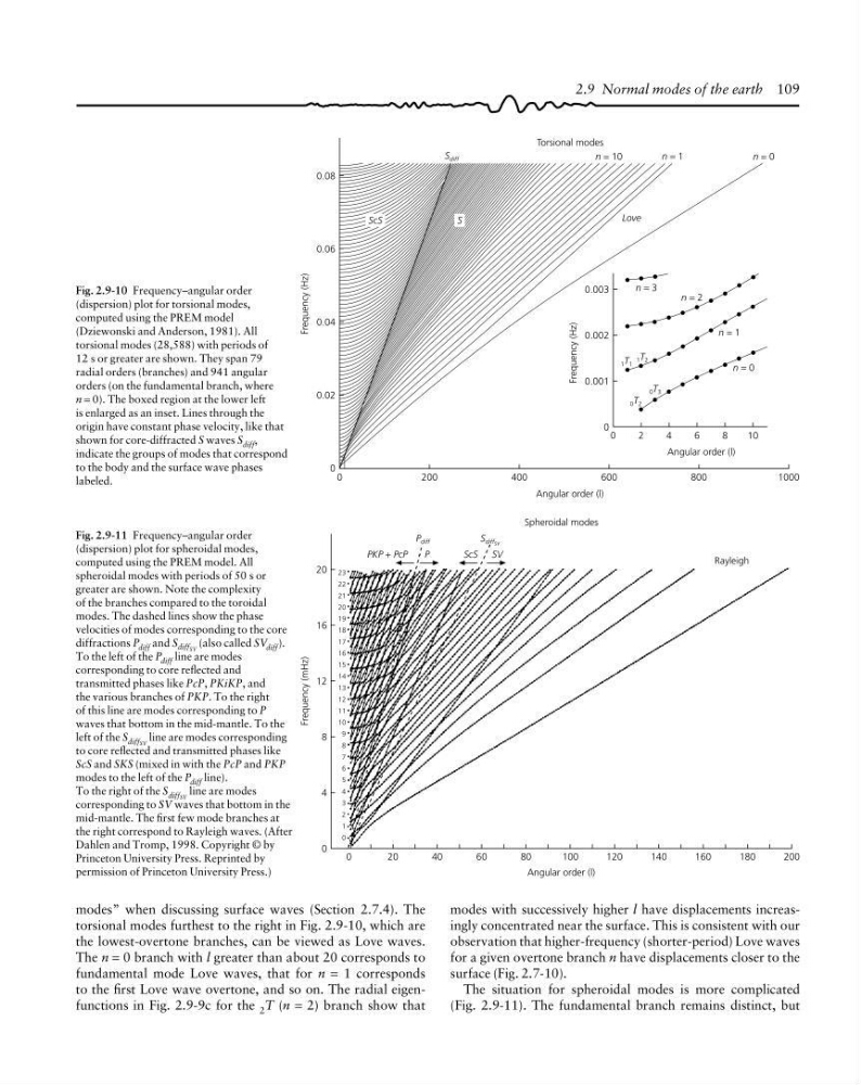
Fig. 2.9-11 Frequency–angular order
(dispersion) plot for spheroidal modes,
computed using the PREM model. All
spheroidal modes with periods of 50 s or
greater are shown. Note the complexity
of the branches compared to the toroidal
modes. The dashed lines show the phase
velocities of modes corresponding to the core
diffractions P diff and S diff SV (also called SV diff ).
To the left of the P diff line are modes
corresponding to core reflected and
transmitted phases like PcP, PKiKP, and
the various branches of PKP. To the right
of this line are modes corresponding to P
waves that bottom in the mid-mantle. To the
left of the S diffSV line are modes corresponding
to core reflected and transmitted phases like
ScS and SKS (mixed in with the PcP and PKP
modes to the left of the P diff line).
To the right of the S diffSV line are modes
corresponding to SV waves that bottom in the
mid-mantle. The first few mode branches at
the right correspond to Rayleigh waves. (After
Dahlen and Tromp, 1998. Copyright © by
Princeton University Press. Reprinted by
permission of Princeton University Press.)
2.9 Normal modes of the earth 109
Frequency (mHz)
20
16
12
8
4
0
200
180
160
140
120
100
80
60
40
20
0
PKP + PcP
P
ScS SV
P diff
S diffsv
23
22
21
20
19
18
17
16
15
14
13
12
11
10
9
8
7
6
5
4
3
2
1
0
Rayleigh
Angular order (l)
Spheroidal modes
modes” when discussing surface waves (Section 2.7.4). The
torsional modes furthest to the right in Fig. 2.9-10, which are
the lowest-overtone branches, can be viewed as Love waves.
The n = 0 branch with l greater than about 20 corresponds to
fundamental mode Love waves, that for n = 1 corresponds
to the first Love wave overtone, and so on. The radial eigenfunctions in Fig. 2.9-9c for the 2 T (n = 2) branch show that
modes with successively higher l have displacements increasingly concentrated near the surface. This is consistent with our
observation that higher-frequency (shorter-period) Love waves
for a given overtone branch n have displacements closer to the
surface (Fig. 2.7-10).
The situation for spheroidal modes is more complicated
(Fig. 2.9-11). The fundamental branch remains distinct, but
Fig. 2.9-10 Frequency–angular order
(dispersion) plot for torsional modes,
computed using the PREM model
(Dziewonski and Anderson, 1981). All
torsional modes (28,588) with periods of
12 s or greater are shown. They span 79
radial orders (branches) and 941 angular
orders (on the fundamental branch, where
n = 0). The boxed region at the lower left
is enlarged as an inset. Lines through the
origin have constant phase velocity, like that
shown for core-diffracted S waves S diff ,
indicate the groups of modes that correspond
to the body and the surface wave phases
labeled.
0.08
0.06
0.04
0.02
0
0
Angular order (l)
S diff
1000
Frequency (Hz)
0.003
0.002
0.001
0
0
Angular order (l)
0 T 2
10
200
600
800
400
2
4
6
8
0 T 3
1 T 2
1 T 1
n = 3
n = 2
n = 1
n = 0
Love
S
ScS
n = 10
n = 1
n = 0
Torsional modes
Fig. 2.9-11 Frequency–angular order
(dispersion) plot for spheroidal modes,
computed using the PREM model. All
spheroidal modes with periods of 50 s or
greater are shown. Note the complexity
of the branches compared to the toroidal
modes. The dashed lines show the phase
velocities of modes corresponding to the core
diffractions P diff and S diff SV (also called SV diff ).
To the left of the P diff line are modes
corresponding to core reflected and
transmitted phases like PcP, PKiKP, and
the various branches of PKP. To the right
of this line are modes corresponding to P
waves that bottom in the mid-mantle. To the
left of the S diffSV line are modes corresponding
to core reflected and transmitted phases like
ScS and SKS (mixed in with the PcP and PKP
modes to the left of the P diff line).
To the right of the S diffSV line are modes
corresponding to SV waves that bottom in the
mid-mantle. The first few mode branches at
the right correspond to Rayleigh waves. (After
Dahlen and Tromp, 1998. Copyright © by
Princeton University Press. Reprinted by
permission of Princeton University Press.)
2.9 Normal modes of the earth 109
Frequency (mHz)
20
16
12
8
4
0
200
180
160
140
120
100
80
60
40
20
0
PKP + PcP
P
ScS SV
P diff
S diffsv
23
22
21
20
19
18
17
16
15
14
13
12
11
10
9
8
7
6
5
4
3
2
1
0
Rayleigh
Angular order (l)
Spheroidal modes
modes” when discussing surface waves (Section 2.7.4). The
torsional modes furthest to the right in Fig. 2.9-10, which are
the lowest-overtone branches, can be viewed as Love waves.
The n = 0 branch with l greater than about 20 corresponds to
fundamental mode Love waves, that for n = 1 corresponds
to the first Love wave overtone, and so on. The radial eigenfunctions in Fig. 2.9-9c for the 2 T (n = 2) branch show that
modes with successively higher l have displacements increasingly concentrated near the surface. This is consistent with our
observation that higher-frequency (shorter-period) Love waves
for a given overtone branch n have displacements closer to the
surface (Fig. 2.7-10).
The situation for spheroidal modes is more complicated
(Fig. 2.9-11). The fundamental branch remains distinct, but
Fig. 2.9-10 Frequency–angular order
(dispersion) plot for torsional modes,
computed using the PREM model
(Dziewonski and Anderson, 1981). All
torsional modes (28,588) with periods of
12 s or greater are shown. They span 79
radial orders (branches) and 941 angular
orders (on the fundamental branch, where
n = 0). The boxed region at the lower left
is enlarged as an inset. Lines through the
origin have constant phase velocity, like that
shown for core-diffracted S waves S diff ,
indicate the groups of modes that correspond
to the body and the surface wave phases
labeled.