

Taking derivatives of Eqn 18 shows the ratio of the partial
derivatives,
∂
∂
∂
∂
Y
Y
l
m
l
m
( , )
( , )
,
θ φ
θ
θ φ
φ
>> 1
(22)
because l was assumed to be much greater than m. For
torsional modes, the T l
m vector spherical harmonic (Eqn 10)
generally has a φ component greater than its θ component, so
its displacement is primarily perpendicular to the plane connecting the source and the receiver, like an SH or a Love wave
(Fig. 2.9-1). By contrast, the spheroidal mode vector spherical
harmonic S l
m (Eqn 14) generally has a θ component greater
than its φ component, and so causes displacement primarily in
the plane connecting the source and the receiver, like a P–SV or
a Rayleigh wave.
We can use these ideas to relate modes to specific body and
surface wave phases. A good place to start is to recall that for
Love waves in a layer over a halfspace, the boundary conditions at the free surface and the interface require that the Love
wave have discrete eigenfrequencies that depend on the layer
thickness and the shear velocity of the layer and the halfspace.
We thus obtain a dispersion relation (Section 2.7.3) giving the
phase velocity as a function of frequency for these modes.
Because the dispersion relation depends on the earth structure
assumed in computing it, we can compare the observed dispersion of surface waves to the predictions of different earth
models, and invert the observations to derive earth models that
better fit the data (e.g., Fig. 2.8-3).
Analogous computations for the spherical earth predict
the normal mode eigenfunctions and eigenfrequencies, which
depend on the earth model assumed. Figure 2.9-9 shows a plot
of radial eigenfunctions for some modes. As for surface waves,
modes with different eigenfrequencies sample different depths
within the earth. For example, as noted in Fig. 2.9-6, Fig. 2.99A shows that a torsional overtone of order n has n nodal
surfaces at depths determined by the velocity structure of the
mantle. Thus the observed eigenfrequencies can be inverted to
model the earth’s radial velocity structure. This process yields
earth models that match the observed eigenfrequencies quite
well, as illustrated by the dashed line in Fig. 2.9-2. Moreover,
the results can be checked by combining them with travel time
observations. For instance, before PKJKP body waves 6 were
observed, the shear velocity of the inner core was constrained
using normal modes like 10 S 2 that have large displacements in
the inner core.
Figure 2.9-10 shows a plot of the eigenfrequency versus
angular order for torsional modes. The modes plot along distinct lines, corresponding to overtone branches. The lowest line
is the fundamental branch (radial order n = 0) with the lowest
eigenfrequency (longest period) for any given angular order. The
Propagating Rayleigh waves
Earthquake
A few minutes after
the earthquake
A few hours after
the earthquake
Standing waves
(oscillating mode)
0 S 25
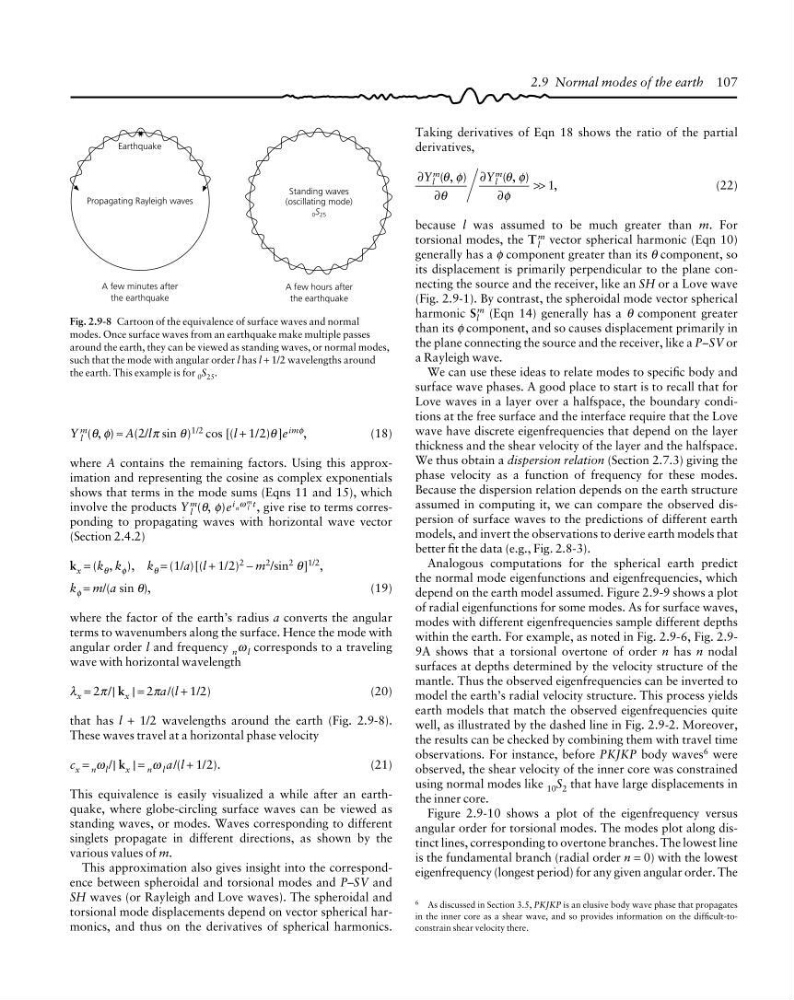
Fig. 2.9-8 Cartoon of the equivalence of surface waves and normal
modes. Once surface waves from an earthquake make multiple passes
around the earth, they can be viewed as standing waves, or normal modes,
such that the mode with angular order l has l + 1/2 wavelengths around
the earth. This example is for 0 S 25 .
6 As discussed in Section 3.5, PKJKP is an elusive body wave phase that propagates
in the inner core as a shear wave, and so provides information on the difficult-toconstrain shear velocity there.
2.9 Normal modes of the earth 107
Y l
m
(θ, φ) ≈ A(2/lπ sin θ)
1/2 cos [(l + 1/2)θ ]e
imφ ,
(18)
where A contains the remaining factors. Using this approximation and representing the cosine as complex exponentials
shows that terms in the mode sums (Eqns 11 and 15), which
involve the products Y l
m (θ, φ)e i n ω l
m t , give rise to terms corresponding to propagating waves with horizontal wave vector
(Section 2.4.2)
k x = (k θ , k φ ), k θ = (1/a)[(l + 1/2) 2 − m 2 /sin 2 θ] 1/2 ,
k φ = m/(a sin θ),
(19)
where the factor of the earth’s radius a converts the angular
terms to wavenumbers along the surface. Hence the mode with
angular order l and frequency n ω l corresponds to a traveling
wave with horizontal wavelength
λ x = 2π /| k x | = 2πa/(l + 1/2)
(20)
that has l + 1/2 wavelengths around the earth (Fig. 2.9-8).
These waves travel at a horizontal phase velocity
c x = n ω l /| k x | = n ω l a/(l + 1/2).
(21)
This equivalence is easily visualized a while after an earthquake, where globe-circling surface waves can be viewed as
standing waves, or modes. Waves corresponding to different
singlets propagate in different directions, as shown by the
various values of m.
This approximation also gives insight into the correspondence between spheroidal and torsional modes and P–SV and
SH waves (or Rayleigh and Love waves). The spheroidal and
torsional mode displacements depend on vector spherical harmonics, and thus on the derivatives of spherical harmonics.
derivatives,
∂
∂
∂
∂
Y
Y
l
m
l
m
( , )
( , )
,
θ φ
θ
θ φ
φ
>> 1
(22)
because l was assumed to be much greater than m. For
torsional modes, the T l
m vector spherical harmonic (Eqn 10)
generally has a φ component greater than its θ component, so
its displacement is primarily perpendicular to the plane connecting the source and the receiver, like an SH or a Love wave
(Fig. 2.9-1). By contrast, the spheroidal mode vector spherical
harmonic S l
m (Eqn 14) generally has a θ component greater
than its φ component, and so causes displacement primarily in
the plane connecting the source and the receiver, like a P–SV or
a Rayleigh wave.
We can use these ideas to relate modes to specific body and
surface wave phases. A good place to start is to recall that for
Love waves in a layer over a halfspace, the boundary conditions at the free surface and the interface require that the Love
wave have discrete eigenfrequencies that depend on the layer
thickness and the shear velocity of the layer and the halfspace.
We thus obtain a dispersion relation (Section 2.7.3) giving the
phase velocity as a function of frequency for these modes.
Because the dispersion relation depends on the earth structure
assumed in computing it, we can compare the observed dispersion of surface waves to the predictions of different earth
models, and invert the observations to derive earth models that
better fit the data (e.g., Fig. 2.8-3).
Analogous computations for the spherical earth predict
the normal mode eigenfunctions and eigenfrequencies, which
depend on the earth model assumed. Figure 2.9-9 shows a plot
of radial eigenfunctions for some modes. As for surface waves,
modes with different eigenfrequencies sample different depths
within the earth. For example, as noted in Fig. 2.9-6, Fig. 2.99A shows that a torsional overtone of order n has n nodal
surfaces at depths determined by the velocity structure of the
mantle. Thus the observed eigenfrequencies can be inverted to
model the earth’s radial velocity structure. This process yields
earth models that match the observed eigenfrequencies quite
well, as illustrated by the dashed line in Fig. 2.9-2. Moreover,
the results can be checked by combining them with travel time
observations. For instance, before PKJKP body waves 6 were
observed, the shear velocity of the inner core was constrained
using normal modes like 10 S 2 that have large displacements in
the inner core.
Figure 2.9-10 shows a plot of the eigenfrequency versus
angular order for torsional modes. The modes plot along distinct lines, corresponding to overtone branches. The lowest line
is the fundamental branch (radial order n = 0) with the lowest
eigenfrequency (longest period) for any given angular order. The
Propagating Rayleigh waves
Earthquake
A few minutes after
the earthquake
A few hours after
the earthquake
Standing waves
(oscillating mode)
0 S 25
Fig. 2.9-8 Cartoon of the equivalence of surface waves and normal
modes. Once surface waves from an earthquake make multiple passes
around the earth, they can be viewed as standing waves, or normal modes,
such that the mode with angular order l has l + 1/2 wavelengths around
the earth. This example is for 0 S 25 .
6 As discussed in Section 3.5, PKJKP is an elusive body wave phase that propagates
in the inner core as a shear wave, and so provides information on the difficult-toconstrain shear velocity there.
2.9 Normal modes of the earth 107
Y l
m
(θ, φ) ≈ A(2/lπ sin θ)
1/2 cos [(l + 1/2)θ ]e
imφ ,
(18)
where A contains the remaining factors. Using this approximation and representing the cosine as complex exponentials
shows that terms in the mode sums (Eqns 11 and 15), which
involve the products Y l
m (θ, φ)e i n ω l
m t , give rise to terms corresponding to propagating waves with horizontal wave vector
(Section 2.4.2)
k x = (k θ , k φ ), k θ = (1/a)[(l + 1/2) 2 − m 2 /sin 2 θ] 1/2 ,
k φ = m/(a sin θ),
(19)
where the factor of the earth’s radius a converts the angular
terms to wavenumbers along the surface. Hence the mode with
angular order l and frequency n ω l corresponds to a traveling
wave with horizontal wavelength
λ x = 2π /| k x | = 2πa/(l + 1/2)
(20)
that has l + 1/2 wavelengths around the earth (Fig. 2.9-8).
These waves travel at a horizontal phase velocity
c x = n ω l /| k x | = n ω l a/(l + 1/2).
(21)
This equivalence is easily visualized a while after an earthquake, where globe-circling surface waves can be viewed as
standing waves, or modes. Waves corresponding to different
singlets propagate in different directions, as shown by the
various values of m.
This approximation also gives insight into the correspondence between spheroidal and torsional modes and P–SV and
SH waves (or Rayleigh and Love waves). The spheroidal and
torsional mode displacements depend on vector spherical harmonics, and thus on the derivatives of spherical harmonics.