

106 Basic Seismological Theory
oscillating in one direction, with deeper shells oscillating in
opposing directions. The mode 0 T 0 has no physical meaning
and is undefined.
2.9.5 Spheroidal modes
P–SV motions are described in a similar way by spheroidal
modes, also known as poloidal modes. These are more complicated than torsional modes, because they combine radial and
transverse motions. The surface eigenfunctions are given by two
other vector spherical harmonics, with (r, θ, φ) components
R l
m = (Y l
m , 0, 0),
S l
m
l
m
l
m
Y
Y
=
⎛
⎝
⎜
⎞
⎠
⎟
,
( , ) ,
sin
( , ) .
0
1
∂
∂
∂
∂
θ φ
θ
θ
θ φ
φ
(14)
Each corresponds to a different radial eigenfunction, n U l (r)
and n V l (r), so the displacement vector u = (u r , u θ , u φ ) for
spheroidal modes is
u
R
S
S
n l
n l
m
n l
l
m
n l
l
m
i
t
m l
l
r
A Ur
V r
e n l
m
( , , )
[ ( ) ( , )
( ) ( , )]
.
θ φ
θ φ
θ φ
ω
=
+
∑ ∑ ∑
=−
(15)
Thus the radial eigenfunction n U l (r) corresponds to radial
motion, and n V l (r) corresponds to horizontal motion.
To see that the mode formulation separates P–SV from SH
and fully represents the displacement in three dimensions, note
that the three vector spherical harmonics are orthogonal,
T l
m · S l
m = T l
m · R l
m = S l
m · R l
m = 0.
(16)
Spheroidal modes n S l
m follow a similar nomenclature as torsional modes. The fundamental modes, with no internal nodal
surfaces, are described by n = 0. As n increases, the number of
internal nodal surfaces increases, although, unlike for torsional
modes, n is not the number of nodal surfaces. The angular
order l equals the number of nodal lines at the surface (rather
than l − 1 for torsional modes), and m represents the number
of great circle nodal lines passing through the pole. The spheroidal radial modes, which have l = 0 and thus only radial
motions, have no torsional analogue.
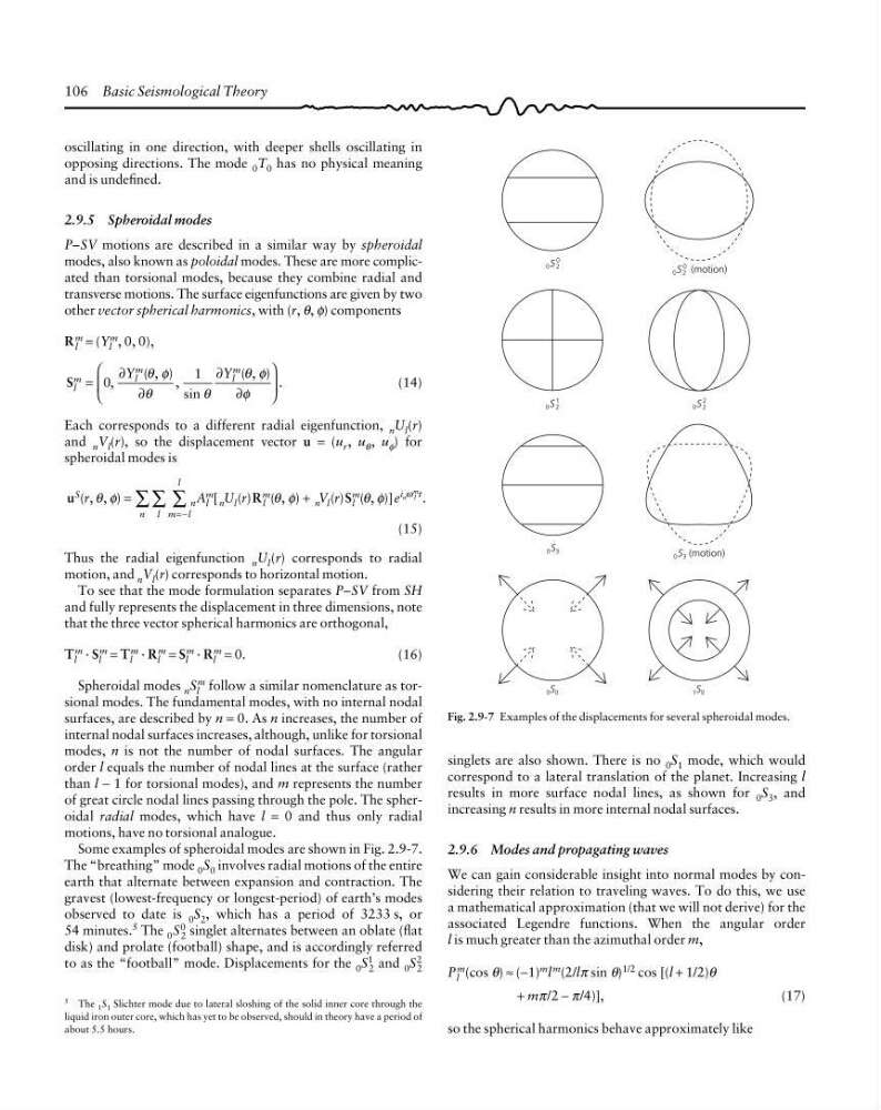
Some examples of spheroidal modes are shown in Fig. 2.9-7.
The “breathing” mode 0 S 0 involves radial motions of the entire
earth that alternate between expansion and contraction. The
gravest (lowest-frequency or longest-period) of earth’s modes
observed to date is 0 S 2 , which has a period of 3233 s, or
54 minutes. 5 The 0 S 0
2 singlet alternates between an oblate (flat
disk) and prolate (football) shape, and is accordingly referred
to as the “football” mode. Displacements for the 0 S 1
2 and 0 S 2
2
Fig. 2.9-7 Examples of the displacements for several spheroidal modes.
0 S 2
0 (motion)
0 S 2
0
0 S 2
1
0 S 2
2
0 S 3
0 S 0
1 S 0
0 S 3 (motion)
5 The 1 S 1 Slichter mode due to lateral sloshing of the solid inner core through the
liquid iron outer core, which has yet to be observed, should in theory have a period of
about 5.5 hours.
singlets are also shown. There is no 0 S 1 mode, which would
correspond to a lateral translation of the planet. Increasing l
results in more surface nodal lines, as shown for 0 S 3 , and
increasing n results in more internal nodal surfaces.
2.9.6 Modes and propagating waves
We can gain considerable insight into normal modes by considering their relation to traveling waves. To do this, we use
a mathematical approximation (that we will not derive) for the
associated Legendre functions. When the angular order
l is much greater than the azimuthal order m,
P l
m (cos θ) ≈ (−1)
m l
m
(2/lπ sin θ)
1/2 cos [(l + 1/2)θ
+ mπ/2 − π/4)],
(17)
so the spherical harmonics behave approximately like
oscillating in one direction, with deeper shells oscillating in
opposing directions. The mode 0 T 0 has no physical meaning
and is undefined.
2.9.5 Spheroidal modes
P–SV motions are described in a similar way by spheroidal
modes, also known as poloidal modes. These are more complicated than torsional modes, because they combine radial and
transverse motions. The surface eigenfunctions are given by two
other vector spherical harmonics, with (r, θ, φ) components
R l
m = (Y l
m , 0, 0),
S l
m
l
m
l
m
Y
Y
=
⎛
⎝
⎜
⎞
⎠
⎟
,
( , ) ,
sin
( , ) .
0
1
∂
∂
∂
∂
θ φ
θ
θ
θ φ
φ
(14)
Each corresponds to a different radial eigenfunction, n U l (r)
and n V l (r), so the displacement vector u = (u r , u θ , u φ ) for
spheroidal modes is
u
R
S
S
n l
n l
m
n l
l
m
n l
l
m
i
t
m l
l
r
A Ur
V r
e n l
m
( , , )
[ ( ) ( , )
( ) ( , )]
.
θ φ
θ φ
θ φ
ω
=
+
∑ ∑ ∑
=−
(15)
Thus the radial eigenfunction n U l (r) corresponds to radial
motion, and n V l (r) corresponds to horizontal motion.
To see that the mode formulation separates P–SV from SH
and fully represents the displacement in three dimensions, note
that the three vector spherical harmonics are orthogonal,
T l
m · S l
m = T l
m · R l
m = S l
m · R l
m = 0.
(16)
Spheroidal modes n S l
m follow a similar nomenclature as torsional modes. The fundamental modes, with no internal nodal
surfaces, are described by n = 0. As n increases, the number of
internal nodal surfaces increases, although, unlike for torsional
modes, n is not the number of nodal surfaces. The angular
order l equals the number of nodal lines at the surface (rather
than l − 1 for torsional modes), and m represents the number
of great circle nodal lines passing through the pole. The spheroidal radial modes, which have l = 0 and thus only radial
motions, have no torsional analogue.
Some examples of spheroidal modes are shown in Fig. 2.9-7.
The “breathing” mode 0 S 0 involves radial motions of the entire
earth that alternate between expansion and contraction. The
gravest (lowest-frequency or longest-period) of earth’s modes
observed to date is 0 S 2 , which has a period of 3233 s, or
54 minutes. 5 The 0 S 0
2 singlet alternates between an oblate (flat
disk) and prolate (football) shape, and is accordingly referred
to as the “football” mode. Displacements for the 0 S 1
2 and 0 S 2
2
Fig. 2.9-7 Examples of the displacements for several spheroidal modes.
0 S 2
0 (motion)
0 S 2
0
0 S 2
1
0 S 2
2
0 S 3
0 S 0
1 S 0
0 S 3 (motion)
5 The 1 S 1 Slichter mode due to lateral sloshing of the solid inner core through the
liquid iron outer core, which has yet to be observed, should in theory have a period of
about 5.5 hours.
singlets are also shown. There is no 0 S 1 mode, which would
correspond to a lateral translation of the planet. Increasing l
results in more surface nodal lines, as shown for 0 S 3 , and
increasing n results in more internal nodal surfaces.
2.9.6 Modes and propagating waves
We can gain considerable insight into normal modes by considering their relation to traveling waves. To do this, we use
a mathematical approximation (that we will not derive) for the
associated Legendre functions. When the angular order
l is much greater than the azimuthal order m,
P l
m (cos θ) ≈ (−1)
m l
m
(2/lπ sin θ)
1/2 cos [(l + 1/2)θ
+ mπ/2 − π/4)],
(17)
so the spherical harmonics behave approximately like