

104 Basic Seismological Theory
2.9.4 Torsional modes
Using spherical harmonics, we can write the normal modes of
a sphere (Eqn 4) explicitly. You may recall that in Cartesian
coordinates we separated the displacements into P–SV and SH
motions, which are decoupled in the sense that they propagate
independently in a medium whose properties vary only in
depth along the plane containing the source and the receiver
(Section 2.5.2). In spherical geometry, we do a similar decomposition with normal modes.
Analogous to SH waves, we have torsional, or toroidal,
modes. Their surface eigenfunctions are given by the vector
spherical harmonics with (r, θ, φ) components
T l
m
l
m
l
m
Y
Y
=
⎛
⎝
⎜
⎞
⎠
⎟
,
sin
( , ) ,
( , ) .
0
1
θ
θ φ
φ
θ φ
θ
∂
∂
−∂
∂
(10)
The vector spherical harmonics are vectors whose components
contain derivatives of spherical harmonics, which arise because
the equation of motion involves spatial derivatives of the
displacements.
The displacement vector u = (u r , u θ , u φ ) that corresponds to
torsional modes is
u
T
T
n l
n
m
n l
l
m
i
t
m l
l
r
A W r
e n l
m
( , , )
( )
( , )
.
θ φ
θ φ
ω
= ∑ ∑ ∑
= −
l
(11)
The radial eigenfunction n W l (r) varies with depth, even though
the resulting displacement has no radial component because u r
is always zero. Thus torsional modes have only horizontal
displacements and are analogous to SH waves. Similarly, their
divergence is zero, so they cause no volume change.
Torsional modes are denoted n T l
m , where n is the radial
order, l is the angular order, and m is the azimuthal order.
For given radial and angular orders, the 2l + 1 modes of different azimuthal orders −l ≤ m ≤ l are called singlets, and the
group of singlets is called a multiplet. If the earth were perfectly
spherically symmetric, and not rotating, then all the singlets in
a multiplet would have the same eigenfrequency. This condition is called degeneracy. For example, the period of n T l
0 would
be the same for n T l
±1 , n T l
±2 , n T l
±3 , etc. In the real earth, the
singlet frequencies vary, which is an effect called splitting.
However, the splitting is small enough that for most applications we ignore it, dropping the m superscript and referring
to the entire n T l
m multiplet as n T l , with eigenfrequency n ω l .
For torsional modes, the horizontal displacements, u θ and u φ ,
are zero along nodal lines, because the angular displacements
u θ vanish where ∂Y l
m
/ ∂φ = 0 and the azimuthal displacements u φ
vanish where ∂Y l
m / ∂θ = 0. For example, consider the lowestfrequency (longest-period or gravest) torsional normal mode
singlet, 0 T 2
0 (Fig. 2.9-5). There are no radial motions, and the
angular displacements are always zero, because m = 0. To see
this, note, from Eqn 10, that u θ is proportional to
Re(Y
2
4 )
Re(Y
3
3 )
Y
0
2
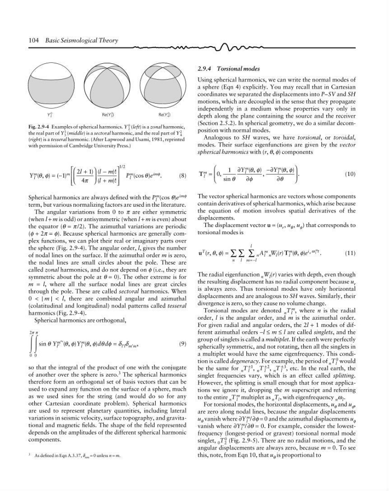
Fig. 2.9-4 Examples of spherical harmonics. Y
0
2 (left) is a zonal harmonic,
the real part of Y
3
3 (middle) is a sectoral harmonic, and the real part of Y
2
4
(right) is a tesseral harmonic. (After Lapwood and Usami, 1981, reprinted
with permission of Cambridge University Press.)
3 As defined in Eqn A.3.37, δ nm = 0 unless n = m.
Y
l
l m
l m
P
e
l
m
m
l
m
i m
( , ) ( )
) (
)!
(
)!
(cos )
.
/
θ φ
π
θ
φ
= −
+
⎛
⎝
⎜
⎞
⎠
⎟
−
+
⎡
⎣
⎢
⎢
⎤
⎦
⎥
⎥
1
2 1
4
1 2
(8)
Spherical harmonics are always defined with the P l
m (cos θ)e imφ
term, but various normalizing factors are used in the literature.
The angular variations from 0 to π are either symmetric
(when l + m is odd) or antisymmetric (when l + m is even) about
the equator (θ = π /2). The azimuthal variations are periodic
(φ + 2π = φ). Because spherical harmonics are generally complex functions, we can plot their real or imaginary parts over
the sphere (Fig. 2.9-4). The angular order, l, gives the number
of nodal lines on the surface. If the azimuthal order m is zero,
the nodal lines are small circles about the pole. These are
called zonal harmonics, and do not depend on φ (i.e., they are
symmetric about the pole at θ = 0). The other extreme is for
m = l, where all the surface nodal lines are great circles
through the pole. These are called sectoral harmonics. When
0 < | m | < l, there are combined angular and azimuthal
(colatitudinal and longitudinal) nodal patterns called tesseral
harmonics (Fig. 2.9-4).
Spherical harmonics are orthogonal,
ΎΎ
0
2
0
π π
θ
θ φ
θ φ θ φ δ δ
sin
( , ) ( , )
,
*
Y
Y
d d
l
m
l
m
l l m m
′
′
′
′
=
(9)
so that the integral of the product of one with the conjugate
of another over the sphere is zero.
3 The spherical harmonics
therefore form an orthogonal set of basis vectors that can be
used to expand any function on the surface of a sphere, much
as we used sines for the string (and would do so for any
other Cartesian coordinate problem). Spherical harmonics
are used to represent planetary quantities, including lateral
variations in seismic velocity, surface topography, and gravitational and magnetic fields. The shape of the field represented
depends on the amplitudes of the different spherical harmonic
components.
2.9.4 Torsional modes
Using spherical harmonics, we can write the normal modes of
a sphere (Eqn 4) explicitly. You may recall that in Cartesian
coordinates we separated the displacements into P–SV and SH
motions, which are decoupled in the sense that they propagate
independently in a medium whose properties vary only in
depth along the plane containing the source and the receiver
(Section 2.5.2). In spherical geometry, we do a similar decomposition with normal modes.
Analogous to SH waves, we have torsional, or toroidal,
modes. Their surface eigenfunctions are given by the vector
spherical harmonics with (r, θ, φ) components
T l
m
l
m
l
m
Y
Y
=
⎛
⎝
⎜
⎞
⎠
⎟
,
sin
( , ) ,
( , ) .
0
1
θ
θ φ
φ
θ φ
θ
∂
∂
−∂
∂
(10)
The vector spherical harmonics are vectors whose components
contain derivatives of spherical harmonics, which arise because
the equation of motion involves spatial derivatives of the
displacements.
The displacement vector u = (u r , u θ , u φ ) that corresponds to
torsional modes is
u
T
T
n l
n
m
n l
l
m
i
t
m l
l
r
A W r
e n l
m
( , , )
( )
( , )
.
θ φ
θ φ
ω
= ∑ ∑ ∑
= −
l
(11)
The radial eigenfunction n W l (r) varies with depth, even though
the resulting displacement has no radial component because u r
is always zero. Thus torsional modes have only horizontal
displacements and are analogous to SH waves. Similarly, their
divergence is zero, so they cause no volume change.
Torsional modes are denoted n T l
m , where n is the radial
order, l is the angular order, and m is the azimuthal order.
For given radial and angular orders, the 2l + 1 modes of different azimuthal orders −l ≤ m ≤ l are called singlets, and the
group of singlets is called a multiplet. If the earth were perfectly
spherically symmetric, and not rotating, then all the singlets in
a multiplet would have the same eigenfrequency. This condition is called degeneracy. For example, the period of n T l
0 would
be the same for n T l
±1 , n T l
±2 , n T l
±3 , etc. In the real earth, the
singlet frequencies vary, which is an effect called splitting.
However, the splitting is small enough that for most applications we ignore it, dropping the m superscript and referring
to the entire n T l
m multiplet as n T l , with eigenfrequency n ω l .
For torsional modes, the horizontal displacements, u θ and u φ ,
are zero along nodal lines, because the angular displacements
u θ vanish where ∂Y l
m
/ ∂φ = 0 and the azimuthal displacements u φ
vanish where ∂Y l
m / ∂θ = 0. For example, consider the lowestfrequency (longest-period or gravest) torsional normal mode
singlet, 0 T 2
0 (Fig. 2.9-5). There are no radial motions, and the
angular displacements are always zero, because m = 0. To see
this, note, from Eqn 10, that u θ is proportional to
Re(Y
2
4 )
Re(Y
3
3 )
Y
0
2
Fig. 2.9-4 Examples of spherical harmonics. Y
0
2 (left) is a zonal harmonic,
the real part of Y
3
3 (middle) is a sectoral harmonic, and the real part of Y
2
4
(right) is a tesseral harmonic. (After Lapwood and Usami, 1981, reprinted
with permission of Cambridge University Press.)
3 As defined in Eqn A.3.37, δ nm = 0 unless n = m.
Y
l
l m
l m
P
e
l
m
m
l
m
i m
( , ) ( )
) (
)!
(
)!
(cos )
.
/
θ φ
π
θ
φ
= −
+
⎛
⎝
⎜
⎞
⎠
⎟
−
+
⎡
⎣
⎢
⎢
⎤
⎦
⎥
⎥
1
2 1
4
1 2
(8)
Spherical harmonics are always defined with the P l
m (cos θ)e imφ
term, but various normalizing factors are used in the literature.
The angular variations from 0 to π are either symmetric
(when l + m is odd) or antisymmetric (when l + m is even) about
the equator (θ = π /2). The azimuthal variations are periodic
(φ + 2π = φ). Because spherical harmonics are generally complex functions, we can plot their real or imaginary parts over
the sphere (Fig. 2.9-4). The angular order, l, gives the number
of nodal lines on the surface. If the azimuthal order m is zero,
the nodal lines are small circles about the pole. These are
called zonal harmonics, and do not depend on φ (i.e., they are
symmetric about the pole at θ = 0). The other extreme is for
m = l, where all the surface nodal lines are great circles
through the pole. These are called sectoral harmonics. When
0 < | m | < l, there are combined angular and azimuthal
(colatitudinal and longitudinal) nodal patterns called tesseral
harmonics (Fig. 2.9-4).
Spherical harmonics are orthogonal,
ΎΎ
0
2
0
π π
θ
θ φ
θ φ θ φ δ δ
sin
( , ) ( , )
,
*
Y
Y
d d
l
m
l
m
l l m m
′
′
′
′
=
(9)
so that the integral of the product of one with the conjugate
of another over the sphere is zero.
3 The spherical harmonics
therefore form an orthogonal set of basis vectors that can be
used to expand any function on the surface of a sphere, much
as we used sines for the string (and would do so for any
other Cartesian coordinate problem). Spherical harmonics
are used to represent planetary quantities, including lateral
variations in seismic velocity, surface topography, and gravitational and magnetic fields. The shape of the field represented
depends on the amplitudes of the different spherical harmonic
components.