

0.36
Frequency (mHz)
0.56
0.76
0.96
1.16
1.36
1.56
1.76
1.96
2.16
4 S 4
1 T 8
2 T 3
0 T 15
7 S 1
2 S 9
0 S 14
2 T 2
5 S 2
0 S 13
0 T 14
1 T 7
4 S 3
2 S 8
0 S 12
6 S 1
1 S 9
0 T 13
0 T 12
0 S 11
2 S 7
5 S 1
4 S 2
0 S 10
0 T 11
1 T 5
0 S 9
1 T 4
0 T 10
1 S 0
2 S 5
1 S 6
4 S 1
0 S 8
1 T 3
0 T 8
1 S 5
2 S 4
0 T 7
1 T 1
0 S 7
2 S 3
1 S 4
3 S 2
0 S 6
1 S 3
3 S 1
0 S 0
0 S 5
1 S 2
0 S 4
0 S 3
1 S 10
5 S 3
2 T 1
1 S 8
1 S 7
2 S 6
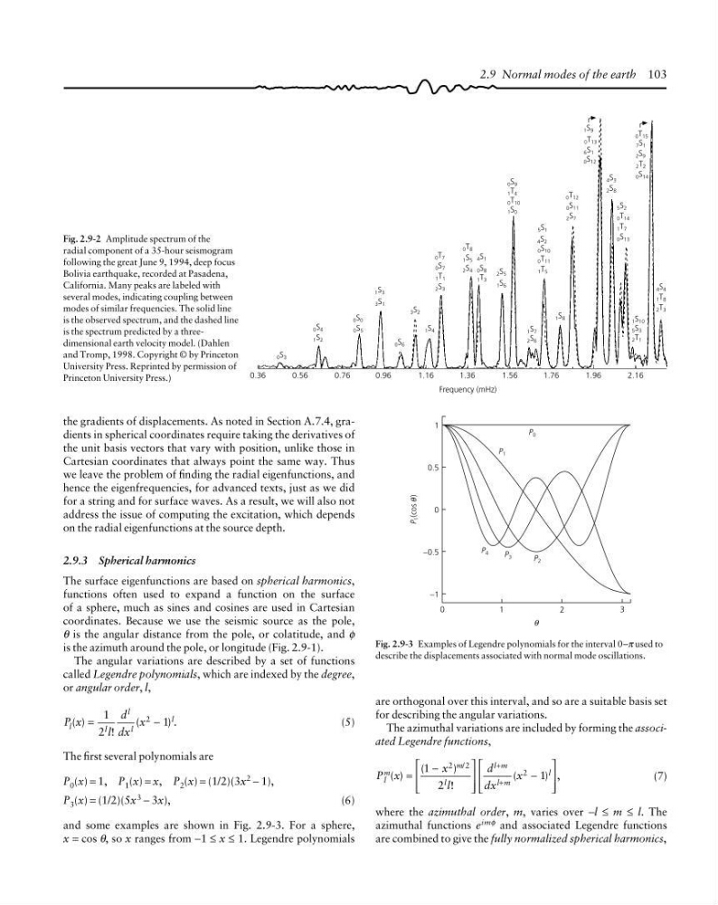
Fig. 2.9-2 Amplitude spectrum of the
radial component of a 35-hour seismogram
following the great June 9, 1994, deep focus
Bolivia earthquake, recorded at Pasadena,
California. Many peaks are labeled with
several modes, indicating coupling between
modes of similar frequencies. The solid line
is the observed spectrum, and the dashed line
is the spectrum predicted by a threedimensional earth velocity model. (Dahlen
and Tromp, 1998. Copyright © by Princeton
University Press. Reprinted by permission of
Princeton University Press.)
2.9 Normal modes of the earth 103
the gradients of displacements. As noted in Section A.7.4, gradients in spherical coordinates require taking the derivatives of
the unit basis vectors that vary with position, unlike those in
Cartesian coordinates that always point the same way. Thus
we leave the problem of finding the radial eigenfunctions, and
hence the eigenfrequencies, for advanced texts, just as we did
for a string and for surface waves. As a result, we will also not
address the issue of computing the excitation, which depends
on the radial eigenfunctions at the source depth.
2.9.3 Spherical harmonics
The surface eigenfunctions are based on spherical harmonics,
functions often used to expand a function on the surface
of a sphere, much as sines and cosines are used in Cartesian
coordinates. Because we use the seismic source as the pole,
θ is the angular distance from the pole, or colatitude, and φ
is the azimuth around the pole, or longitude (Fig. 2.9-1).
The angular variations are described by a set of functions
called Legendre polynomials, which are indexed by the degree,
or angular order, l,
P x
l
d
dx
x
l
l
l
l
l
( )
!
(
).
=
−
1
2
1
2
(5)
The first several polynomials are
P 0 (x) = 1, P 1 (x) = x, P 2 (x) = (1/2)(3x 2 − 1),
P 3 (x) = (1/2)(5x 3 − 3x),
(6)
and some examples are shown in Fig. 2.9-3. For a sphere,
x = cos θ, so x ranges from −1 ≤ x ≤ 1. Legendre polynomials
P 4
1
0.5
0
−0.5
−1
P
1 (cos )
θ
P 3
P 2
P 0
P 1
0
2
3
1
θ
Fig. 2.9-3 Examples of Legendre polynomials for the interval 0–π used to
describe the displacements associated with normal mode oscillations.
are orthogonal over this interval, and so are a suitable basis set
for describing the angular variations.
The azimuthal variations are included by forming the associated Legendre functions,
P x
x
l
d
dx
x
l
m
m
l
l m
l m
l
( )
(
)
!
(
) ,
/
=
−
⎡
⎣
⎢
⎢
⎤
⎦
⎥
⎥
−
⎡
⎣
⎢
⎢
⎤
⎦
⎥
⎥
+
+
1
2
1
2
2
2
(7)
where the azimuthal order, m, varies over −l ≤ m ≤ l. The
azimuthal functions e imφ and associated Legendre functions
are combined to give the fully normalized spherical harmonics,
Frequency (mHz)
0.56
0.76
0.96
1.16
1.36
1.56
1.76
1.96
2.16
4 S 4
1 T 8
2 T 3
0 T 15
7 S 1
2 S 9
0 S 14
2 T 2
5 S 2
0 S 13
0 T 14
1 T 7
4 S 3
2 S 8
0 S 12
6 S 1
1 S 9
0 T 13
0 T 12
0 S 11
2 S 7
5 S 1
4 S 2
0 S 10
0 T 11
1 T 5
0 S 9
1 T 4
0 T 10
1 S 0
2 S 5
1 S 6
4 S 1
0 S 8
1 T 3
0 T 8
1 S 5
2 S 4
0 T 7
1 T 1
0 S 7
2 S 3
1 S 4
3 S 2
0 S 6
1 S 3
3 S 1
0 S 0
0 S 5
1 S 2
0 S 4
0 S 3
1 S 10
5 S 3
2 T 1
1 S 8
1 S 7
2 S 6
Fig. 2.9-2 Amplitude spectrum of the
radial component of a 35-hour seismogram
following the great June 9, 1994, deep focus
Bolivia earthquake, recorded at Pasadena,
California. Many peaks are labeled with
several modes, indicating coupling between
modes of similar frequencies. The solid line
is the observed spectrum, and the dashed line
is the spectrum predicted by a threedimensional earth velocity model. (Dahlen
and Tromp, 1998. Copyright © by Princeton
University Press. Reprinted by permission of
Princeton University Press.)
2.9 Normal modes of the earth 103
the gradients of displacements. As noted in Section A.7.4, gradients in spherical coordinates require taking the derivatives of
the unit basis vectors that vary with position, unlike those in
Cartesian coordinates that always point the same way. Thus
we leave the problem of finding the radial eigenfunctions, and
hence the eigenfrequencies, for advanced texts, just as we did
for a string and for surface waves. As a result, we will also not
address the issue of computing the excitation, which depends
on the radial eigenfunctions at the source depth.
2.9.3 Spherical harmonics
The surface eigenfunctions are based on spherical harmonics,
functions often used to expand a function on the surface
of a sphere, much as sines and cosines are used in Cartesian
coordinates. Because we use the seismic source as the pole,
θ is the angular distance from the pole, or colatitude, and φ
is the azimuth around the pole, or longitude (Fig. 2.9-1).
The angular variations are described by a set of functions
called Legendre polynomials, which are indexed by the degree,
or angular order, l,
P x
l
d
dx
x
l
l
l
l
l
( )
!
(
).
=
−
1
2
1
2
(5)
The first several polynomials are
P 0 (x) = 1, P 1 (x) = x, P 2 (x) = (1/2)(3x 2 − 1),
P 3 (x) = (1/2)(5x 3 − 3x),
(6)
and some examples are shown in Fig. 2.9-3. For a sphere,
x = cos θ, so x ranges from −1 ≤ x ≤ 1. Legendre polynomials
P 4
1
0.5
0
−0.5
−1
P
1 (cos )
θ
P 3
P 2
P 0
P 1
0
2
3
1
θ
Fig. 2.9-3 Examples of Legendre polynomials for the interval 0–π used to
describe the displacements associated with normal mode oscillations.
are orthogonal over this interval, and so are a suitable basis set
for describing the angular variations.
The azimuthal variations are included by forming the associated Legendre functions,
P x
x
l
d
dx
x
l
m
m
l
l m
l m
l
( )
(
)
!
(
) ,
/
=
−
⎡
⎣
⎢
⎢
⎤
⎦
⎥
⎥
−
⎡
⎣
⎢
⎢
⎤
⎦
⎥
⎥
+
+
1
2
1
2
2
2
(7)
where the azimuthal order, m, varies over −l ≤ m ≤ l. The
azimuthal functions e imφ and associated Legendre functions
are combined to give the fully normalized spherical harmonics,