

102 Basic Seismological Theory
Additional insight into the earth’s modes comes from the
two-dimensional problem of Love waves in a layer over a
halfspace (Section 2.7.3). The medium was semi-infinite,
extending vertically from the surface to all depths, and horizontally in both directions. We wrote a solution of the wave
equation in both the layer and the halfspace as the product of
separate terms describing the vertical and horizontal behaviors.
We then used boundary conditions of zero traction at the free
surface, continuity of traction and displacement at the interface, and energy decaying away from the interface downward,
and found that these conditions require that Love waves have
discrete eigenfrequencies that depend on the thickness of the
layer and the shear velocity of the layer and the halfspace. Each
of these eigenfrequencies thus corresponds to a vertical and
horizontal eigenfunction. Interestingly, the eigenfrequencies
form discrete overtone branches (Fig. 2.7-9), so that for a given
apparent velocity there are several possible eigenfrequencies.
Because the medium is two-dimensional, we need two parameters to list all the eigenfrequencies. One parameter, the
overtone number, varies discretely (0, 1, 2, . . . ) because the
thickness of the layer gives a discrete dimension. The other parameter, the frequency, varies continuously along an overtone
branch, because the horizontal dimension is infinite.
To extend one- and two-dimensional ideas to wave propagation in the three-dimensional spherical earth, we formulate the
normal mode solution in spherical coordinates (Section A.7).
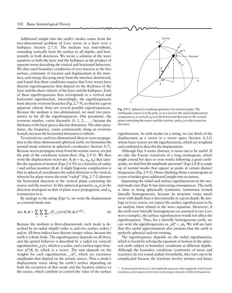
Because waves propagate away from the seismic source, we put
the pole of the coordinate system there (Fig. 2.9-1). We then
write the displacement vector u(r, θ, φ) = (u r , u θ , u φ ) that satisfies the equation of motion (Eqn 2.4.10) as a function of radius
r and surface position (θ, φ). A slight linguistic complication is
that in spherical coordinates the radial direction is the vertical,
whereas for plane waves the term “radial” (Fig. 2.7-2) denotes
the horizontal direction in the vertical plane containing the
source and the receiver. In this spherical geometry, u θ is in the
direction analogous to that of plane wave propagation, and u φ
is transverse to it.
By analogy to the string (Eqn 1), we write the displacement
as a normal mode sum
u
x
( , , )
( ) ( , )
.
r
A yr
e
n l
n
m
n l
l
m
i
t
m
n l
m
θ φ
θ φ
ω
= ∑ ∑ ∑ l
(4)
Because the medium is three-dimensional, each mode is described by its radial (depth) order n, and two surface orders l
and m. All three indices have discrete integer values, because the
earth is a finite body. The eigenfrequency depends on all three,
and the spatial behavior is described by a radial (or vertical)
eigenfunction n y l (r), which is a scalar, and a surface eigen-function x l
m
(θ, φ), which is a vector. The sum depends on the
weights for each eigenfunction, n A l
m , which are excitation
amplitudes that depend on the seismic source. Thus a mode’s
displacement varies along the earth’s surface depending on
both the excitation of that mode and the location relative to
the source, which combine to control the value of the surface
Receiver
Source
x 3
u r
u φ
u θ
θ
φ
r
x 2
x 1
Fig. 2.9-1 Spherical coordinate geometry for normal modes. The
earthquake source is at the pole, so at a receiver the radial displacement
component u r is vertical, u θ is in the horizontal direction in the vertical
plane containing the source and the receiver, and u φ is in the transverse
direction.
2 As discussed in Section 6.2, the amplitude spectrum is the magnitude of the Fourier
transform, and its square shows how much energy is present at different frequencies.
eigenfunction. As with modes on a string, we can think of the
displacement as a vector in a vector space (Section A.3.6)
whose basis vectors are the eigenfunctions, which are weighted
and combined to describe the displacement.
Although Eqn 4 seems abstract, it turns out to be useful. If
we take the Fourier transform of a long seismogram, which
might extend for days or even weeks following a great earthquake, we find that the amplitude spectrum 2 (Eqn 2.8.8) is made
up of normal modes that appear as peaks at certain distinct
frequencies (Fig. 2.9-2). Hence thinking about a seismogram as
a sum of modes gives additional insight into its nature.
Separating the radial and surface eigenfunctions in the normal mode sum (Eqn 4) has interesting consequences. The earth
is close to being spherically symmetric (sometimes termed
laterally homogeneous), because its structure varies much
more with depth than it does laterally at a given depth. By analogy to Love waves, we expect the surface eigenfunction to be
an analytic form related to the wave equation. Moreover, if
the earth were laterally homogeneous (as assumed in our Love
wave example), the surface eigenfunction would not affect the
eigenfrequency. Thus, for a laterally homogeneous earth, we
can write the eigenfrequencies as n ω l
m = n ω l . We will see later
that this useful approximation also assumes that the earth is
perfectly spherical and not rotating.
The eigenfrequency depends on the radial eigenfunction,
which is found by solving the equation of motion in the spherical earth subject to boundary conditions at different depths.
Although the boundary conditions (continuity of stress and
tractions) do not sound unduly formidable, they turn out to be
complicated because the tractions involve stresses and hence
Additional insight into the earth’s modes comes from the
two-dimensional problem of Love waves in a layer over a
halfspace (Section 2.7.3). The medium was semi-infinite,
extending vertically from the surface to all depths, and horizontally in both directions. We wrote a solution of the wave
equation in both the layer and the halfspace as the product of
separate terms describing the vertical and horizontal behaviors.
We then used boundary conditions of zero traction at the free
surface, continuity of traction and displacement at the interface, and energy decaying away from the interface downward,
and found that these conditions require that Love waves have
discrete eigenfrequencies that depend on the thickness of the
layer and the shear velocity of the layer and the halfspace. Each
of these eigenfrequencies thus corresponds to a vertical and
horizontal eigenfunction. Interestingly, the eigenfrequencies
form discrete overtone branches (Fig. 2.7-9), so that for a given
apparent velocity there are several possible eigenfrequencies.
Because the medium is two-dimensional, we need two parameters to list all the eigenfrequencies. One parameter, the
overtone number, varies discretely (0, 1, 2, . . . ) because the
thickness of the layer gives a discrete dimension. The other parameter, the frequency, varies continuously along an overtone
branch, because the horizontal dimension is infinite.
To extend one- and two-dimensional ideas to wave propagation in the three-dimensional spherical earth, we formulate the
normal mode solution in spherical coordinates (Section A.7).
Because waves propagate away from the seismic source, we put
the pole of the coordinate system there (Fig. 2.9-1). We then
write the displacement vector u(r, θ, φ) = (u r , u θ , u φ ) that satisfies the equation of motion (Eqn 2.4.10) as a function of radius
r and surface position (θ, φ). A slight linguistic complication is
that in spherical coordinates the radial direction is the vertical,
whereas for plane waves the term “radial” (Fig. 2.7-2) denotes
the horizontal direction in the vertical plane containing the
source and the receiver. In this spherical geometry, u θ is in the
direction analogous to that of plane wave propagation, and u φ
is transverse to it.
By analogy to the string (Eqn 1), we write the displacement
as a normal mode sum
u
x
( , , )
( ) ( , )
.
r
A yr
e
n l
n
m
n l
l
m
i
t
m
n l
m
θ φ
θ φ
ω
= ∑ ∑ ∑ l
(4)
Because the medium is three-dimensional, each mode is described by its radial (depth) order n, and two surface orders l
and m. All three indices have discrete integer values, because the
earth is a finite body. The eigenfrequency depends on all three,
and the spatial behavior is described by a radial (or vertical)
eigenfunction n y l (r), which is a scalar, and a surface eigen-function x l
m
(θ, φ), which is a vector. The sum depends on the
weights for each eigenfunction, n A l
m , which are excitation
amplitudes that depend on the seismic source. Thus a mode’s
displacement varies along the earth’s surface depending on
both the excitation of that mode and the location relative to
the source, which combine to control the value of the surface
Receiver
Source
x 3
u r
u φ
u θ
θ
φ
r
x 2
x 1
Fig. 2.9-1 Spherical coordinate geometry for normal modes. The
earthquake source is at the pole, so at a receiver the radial displacement
component u r is vertical, u θ is in the horizontal direction in the vertical
plane containing the source and the receiver, and u φ is in the transverse
direction.
2 As discussed in Section 6.2, the amplitude spectrum is the magnitude of the Fourier
transform, and its square shows how much energy is present at different frequencies.
eigenfunction. As with modes on a string, we can think of the
displacement as a vector in a vector space (Section A.3.6)
whose basis vectors are the eigenfunctions, which are weighted
and combined to describe the displacement.
Although Eqn 4 seems abstract, it turns out to be useful. If
we take the Fourier transform of a long seismogram, which
might extend for days or even weeks following a great earthquake, we find that the amplitude spectrum 2 (Eqn 2.8.8) is made
up of normal modes that appear as peaks at certain distinct
frequencies (Fig. 2.9-2). Hence thinking about a seismogram as
a sum of modes gives additional insight into its nature.
Separating the radial and surface eigenfunctions in the normal mode sum (Eqn 4) has interesting consequences. The earth
is close to being spherically symmetric (sometimes termed
laterally homogeneous), because its structure varies much
more with depth than it does laterally at a given depth. By analogy to Love waves, we expect the surface eigenfunction to be
an analytic form related to the wave equation. Moreover, if
the earth were laterally homogeneous (as assumed in our Love
wave example), the surface eigenfunction would not affect the
eigenfrequency. Thus, for a laterally homogeneous earth, we
can write the eigenfrequencies as n ω l
m = n ω l . We will see later
that this useful approximation also assumes that the earth is
perfectly spherical and not rotating.
The eigenfrequency depends on the radial eigenfunction,
which is found by solving the equation of motion in the spherical earth subject to boundary conditions at different depths.
Although the boundary conditions (continuity of stress and
tractions) do not sound unduly formidable, they turn out to be
complicated because the tractions involve stresses and hence