

reasons. First, normal mode calculations are more complicated
than those for rays and plane waves. Second, by representing
all seismic waves simultaneously, mode solutions do not select
specific seismic phases. Hence a phase like ScS emerges from
a computation summing many modes, whereas simpler ray or
plane wave calculations often directly give the information (for
example, travel times and amplitudes) that we seek. However,
there are applications in which modal solutions are useful,
making the topic worthy of study for reasons beyond its physical elegance, although the latter may well be what draws many
seismologists (ourselves included) to it.
2.9.2 Modes of a sphere
The earth’s modes show many features seen for the onedimensional string, so we begin by recalling some basic results.
We saw in Section 2.2.5 that once a one-dimensional string is
excited, its motion can be described as
u x t
A U x
t
n n
n
n
n
( , )
( , ) cos (
),
=
=
∞
∑
ω
ω
0
(1)
which is the sum of standing waves or eigenfunctions,
U n (x, ω n ), each of which is weighted by the amplitude A n
and vibrates at its eigenfrequency ω n . The eigenfunctions and
eigenfrequencies depend on the physical properties of the
string, whereas the amplitudes depend on the position and
nature of the source that excited the motion. We saw that
eigenfunctions that satisfy the wave equation in one dimension
are sine and cosine functions. For a homogeneous (uniform)
string of length L and velocity v, the boundary conditions of
zero displacement at the fixed ends require that
U n (x, ω n ) = sin (nπx/L) = sin (ω n x/v),
(2)
so the eigenfrequencies are
ω n = nπv/L.
(3)
Because the frequency, velocity, and wavelength of a traveling
wave are related by ω = 2πv/λ (Section 2.2.2), Eqn 3 requires
that L = nλ/2, so each spatial eigenfunction has an integral
number of half wavelengths along the string. A finite string can
vibrate only in these discrete modes, which satisfy the boundary conditions. The eigenfrequencies are spaced πv/L apart in
frequency, so if the string were infinite, the eigenfrequencies
would be continuous rather than discrete. Finally, we saw that
the amplitudes depend on the value of the eigenfunction at the
point where the source excited the motion. 1
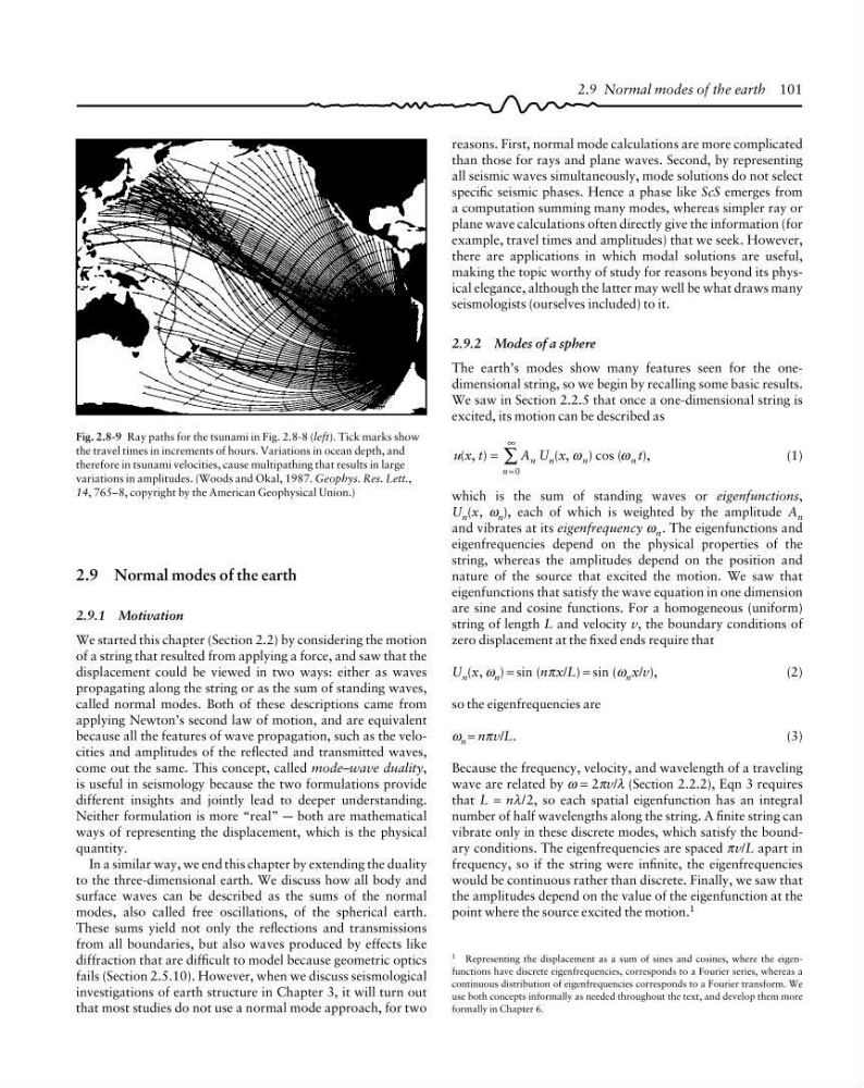
Fig. 2.8-9 Ray paths for the tsunami in Fig. 2.8-8 (left). Tick marks show
the travel times in increments of hours. Variations in ocean depth, and
therefore in tsunami velocities, cause multipathing that results in large
variations in amplitudes. (Woods and Okal, 1987. Geophys. Res. Lett.,
14, 765–8, copyright by the American Geophysical Union.)
2.9 Normal modes of the earth 101
2.9 Normal modes of the earth
2.9.1 Motivation
We started this chapter (Section 2.2) by considering the motion
of a string that resulted from applying a force, and saw that the
displacement could be viewed in two ways: either as waves
propagating along the string or as the sum of standing waves,
called normal modes. Both of these descriptions came from
applying Newton’s second law of motion, and are equivalent
because all the features of wave propagation, such as the velocities and amplitudes of the reflected and transmitted waves,
come out the same. This concept, called mode–wave duality,
is useful in seismology because the two formulations provide
different insights and jointly lead to deeper understanding.
Neither formulation is more “real” — both are mathematical
ways of representing the displacement, which is the physical
quantity.
In a similar way, we end this chapter by extending the duality
to the three-dimensional earth. We discuss how all body and
surface waves can be described as the sums of the normal
modes, also called free oscillations, of the spherical earth.
These sums yield not only the reflections and transmissions
from all boundaries, but also waves produced by effects like
diffraction that are difficult to model because geometric optics
fails (Section 2.5.10). However, when we discuss seismological
investigations of earth structure in Chapter 3, it will turn out
that most studies do not use a normal mode approach, for two
1 Representing the displacement as a sum of sines and cosines, where the eigenfunctions have discrete eigenfrequencies, corresponds to a Fourier series, whereas a
continuous distribution of eigenfrequencies corresponds to a Fourier transform. We
use both concepts informally as needed throughout the text, and develop them more
formally in Chapter 6.
than those for rays and plane waves. Second, by representing
all seismic waves simultaneously, mode solutions do not select
specific seismic phases. Hence a phase like ScS emerges from
a computation summing many modes, whereas simpler ray or
plane wave calculations often directly give the information (for
example, travel times and amplitudes) that we seek. However,
there are applications in which modal solutions are useful,
making the topic worthy of study for reasons beyond its physical elegance, although the latter may well be what draws many
seismologists (ourselves included) to it.
2.9.2 Modes of a sphere
The earth’s modes show many features seen for the onedimensional string, so we begin by recalling some basic results.
We saw in Section 2.2.5 that once a one-dimensional string is
excited, its motion can be described as
u x t
A U x
t
n n
n
n
n
( , )
( , ) cos (
),
=
=
∞
∑
ω
ω
0
(1)
which is the sum of standing waves or eigenfunctions,
U n (x, ω n ), each of which is weighted by the amplitude A n
and vibrates at its eigenfrequency ω n . The eigenfunctions and
eigenfrequencies depend on the physical properties of the
string, whereas the amplitudes depend on the position and
nature of the source that excited the motion. We saw that
eigenfunctions that satisfy the wave equation in one dimension
are sine and cosine functions. For a homogeneous (uniform)
string of length L and velocity v, the boundary conditions of
zero displacement at the fixed ends require that
U n (x, ω n ) = sin (nπx/L) = sin (ω n x/v),
(2)
so the eigenfrequencies are
ω n = nπv/L.
(3)
Because the frequency, velocity, and wavelength of a traveling
wave are related by ω = 2πv/λ (Section 2.2.2), Eqn 3 requires
that L = nλ/2, so each spatial eigenfunction has an integral
number of half wavelengths along the string. A finite string can
vibrate only in these discrete modes, which satisfy the boundary conditions. The eigenfrequencies are spaced πv/L apart in
frequency, so if the string were infinite, the eigenfrequencies
would be continuous rather than discrete. Finally, we saw that
the amplitudes depend on the value of the eigenfunction at the
point where the source excited the motion. 1
Fig. 2.8-9 Ray paths for the tsunami in Fig. 2.8-8 (left). Tick marks show
the travel times in increments of hours. Variations in ocean depth, and
therefore in tsunami velocities, cause multipathing that results in large
variations in amplitudes. (Woods and Okal, 1987. Geophys. Res. Lett.,
14, 765–8, copyright by the American Geophysical Union.)
2.9 Normal modes of the earth 101
2.9 Normal modes of the earth
2.9.1 Motivation
We started this chapter (Section 2.2) by considering the motion
of a string that resulted from applying a force, and saw that the
displacement could be viewed in two ways: either as waves
propagating along the string or as the sum of standing waves,
called normal modes. Both of these descriptions came from
applying Newton’s second law of motion, and are equivalent
because all the features of wave propagation, such as the velocities and amplitudes of the reflected and transmitted waves,
come out the same. This concept, called mode–wave duality,
is useful in seismology because the two formulations provide
different insights and jointly lead to deeper understanding.
Neither formulation is more “real” — both are mathematical
ways of representing the displacement, which is the physical
quantity.
In a similar way, we end this chapter by extending the duality
to the three-dimensional earth. We discuss how all body and
surface waves can be described as the sums of the normal
modes, also called free oscillations, of the spherical earth.
These sums yield not only the reflections and transmissions
from all boundaries, but also waves produced by effects like
diffraction that are difficult to model because geometric optics
fails (Section 2.5.10). However, when we discuss seismological
investigations of earth structure in Chapter 3, it will turn out
that most studies do not use a normal mode approach, for two
1 Representing the displacement as a sum of sines and cosines, where the eigenfunctions have discrete eigenfrequencies, corresponds to a Fourier series, whereas a
continuous distribution of eigenfrequencies corresponds to a Fourier transform. We
use both concepts informally as needed throughout the text, and develop them more
formally in Chapter 6.