

premultiplying both sides, first by the transpose matrix and
then by the inverse of A
T
A,
m = (A T A) −1 A T d.
(29)
The results of such an analysis for Rayleigh wave phase
velocity on many paths crossing the Pacific are shown in
Fig. 2.8-7. As the lithosphere ages, the velocity and the depth
to the low-velocity zone increase, presumably due to the
cooling and thickening of the lithosphere.
Such studies, on both a global and a regional scale, have
contributed greatly to our understanding of the earth’s interior and processes. As we noted, finding velocity structure as
a function of depth from dispersion data is an inverse problem,
which exploits the fact that waves of different periods sample
the structure at depth differently. The pure-path study illustrates a more complicated inverse problem, studying variations
of velocity laterally as well as in depth. Our ability to study
lateral structure comes from the fact that different source–
receiver paths sample different regions. Hence these studies
have the common feature of using observations on the boundaries of a region (either laterally or at depth) to learn about the
structure within it, via observations resulting from sampling
the region in different ways. Such approaches are examples of
tomography, which we will discuss in Chapter 7.
2.8.4 Tsunami dispersion
Dispersion is also observed for tsunamis, the water waves
generated by earthquakes that were discussed in Section 1.2.4.
Tsunamis are like wind-driven water waves, in that they involve
gravitational potential energy stored by vertical displacements
of the water. 2 Although the underlying physics of the propagation differs, there are similarities in the way tsunamis and
surface waves propagate.
As shown in Fig. 2.8-8 (left), tsunami dispersion is similar to
that of Rayleigh and Love waves, in that the waves with longer
periods travel faster and thus arrive earlier. The dispersion
relations (Fig. 2.8-8, right) show two effects that depend on the
period, and thus on the wavelength. At long periods, where the
wavelengths are much greater than the ocean depth, d, the phase
velocities are essentially nondispersive and are given by
c
gd ,
=
(30)
where g is the acceleration of gravity. Thus tsunami velocities depend on ocean depth, as shown. However, at shorter
periods, where the wavelengths are much less than the ocean
depth and so do not “feel” the ocean floor, the tsunami velocities depend on wavelength as
TUC
ARE
4.1
4.0
3.9
3.8
3.7
Phase velocity (km/s)
10
20
30
40
50
60
70
80
90
100
Period (s)
TUC
ARE
Phase dispersion
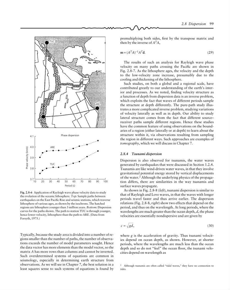
Fig. 2.8-6 Application of Rayleigh wave phase velocity data to study
the evolution of the oceanic lithosphere. Top: Sample paths between
earthquakes on the East Pacific Rise and seismic stations, which traverse
lithosphere of various ages, as shown by the isochrons. The hatched
regions are lithosphere younger than 3 million years. Bottom: Dispersion
curves for the paths shown. The path to station TUC is through younger,
hence lower-velocity, lithosphere than the path to ARE. (Data from
Forsyth, 1975.)
2 Although tsunamis are often called “tidal waves,” they have no connection to
tides.
2.8 Dispersion 99
Typically, because the study area is divided into a number of regions smaller than the number of paths, the number of observations exceeds the number of model parameters sought. Hence
the data vector has more elements than the model vector, so the
matrix A has more rows than columns and cannot be inverted.
Such overdetermined systems of equations are common in
seismology, especially in determining earth structure from
observations. As we will see in Chapter 7, the best solution in a
least squares sense to such systems of equations is found by
then by the inverse of A
T
A,
m = (A T A) −1 A T d.
(29)
The results of such an analysis for Rayleigh wave phase
velocity on many paths crossing the Pacific are shown in
Fig. 2.8-7. As the lithosphere ages, the velocity and the depth
to the low-velocity zone increase, presumably due to the
cooling and thickening of the lithosphere.
Such studies, on both a global and a regional scale, have
contributed greatly to our understanding of the earth’s interior and processes. As we noted, finding velocity structure as
a function of depth from dispersion data is an inverse problem,
which exploits the fact that waves of different periods sample
the structure at depth differently. The pure-path study illustrates a more complicated inverse problem, studying variations
of velocity laterally as well as in depth. Our ability to study
lateral structure comes from the fact that different source–
receiver paths sample different regions. Hence these studies
have the common feature of using observations on the boundaries of a region (either laterally or at depth) to learn about the
structure within it, via observations resulting from sampling
the region in different ways. Such approaches are examples of
tomography, which we will discuss in Chapter 7.
2.8.4 Tsunami dispersion
Dispersion is also observed for tsunamis, the water waves
generated by earthquakes that were discussed in Section 1.2.4.
Tsunamis are like wind-driven water waves, in that they involve
gravitational potential energy stored by vertical displacements
of the water. 2 Although the underlying physics of the propagation differs, there are similarities in the way tsunamis and
surface waves propagate.
As shown in Fig. 2.8-8 (left), tsunami dispersion is similar to
that of Rayleigh and Love waves, in that the waves with longer
periods travel faster and thus arrive earlier. The dispersion
relations (Fig. 2.8-8, right) show two effects that depend on the
period, and thus on the wavelength. At long periods, where the
wavelengths are much greater than the ocean depth, d, the phase
velocities are essentially nondispersive and are given by
c
gd ,
=
(30)
where g is the acceleration of gravity. Thus tsunami velocities depend on ocean depth, as shown. However, at shorter
periods, where the wavelengths are much less than the ocean
depth and so do not “feel” the ocean floor, the tsunami velocities depend on wavelength as
TUC
ARE
4.1
4.0
3.9
3.8
3.7
Phase velocity (km/s)
10
20
30
40
50
60
70
80
90
100
Period (s)
TUC
ARE
Phase dispersion
Fig. 2.8-6 Application of Rayleigh wave phase velocity data to study
the evolution of the oceanic lithosphere. Top: Sample paths between
earthquakes on the East Pacific Rise and seismic stations, which traverse
lithosphere of various ages, as shown by the isochrons. The hatched
regions are lithosphere younger than 3 million years. Bottom: Dispersion
curves for the paths shown. The path to station TUC is through younger,
hence lower-velocity, lithosphere than the path to ARE. (Data from
Forsyth, 1975.)
2 Although tsunamis are often called “tidal waves,” they have no connection to
tides.
2.8 Dispersion 99
Typically, because the study area is divided into a number of regions smaller than the number of paths, the number of observations exceeds the number of model parameters sought. Hence
the data vector has more elements than the model vector, so the
matrix A has more rows than columns and cannot be inverted.
Such overdetermined systems of equations are common in
seismology, especially in determining earth structure from
observations. As we will see in Chapter 7, the best solution in a
least squares sense to such systems of equations is found by