

98 Basic Seismological Theory
−10
−20 −15 −10
−5
0
5
10
15
20
4.8
25
50
75
100
125
150
4.4
4.0
3.6
3.2
Velocity (km/s)
Off-ridge
On-ridge
Depth (km)
Walvis ridge
SDB
Period (s)
90
4.1
4.0
3.9
3.8
3.7
3.6
3.5
3.4
80
70
60
50
40
30
20
10
Walvis ridge
Off ridge-WIN
On ridge-SDB
Mean group dispersion
Group velocity (km/s)
−15
−20
−25
−30
−35
−40
−45
WIN
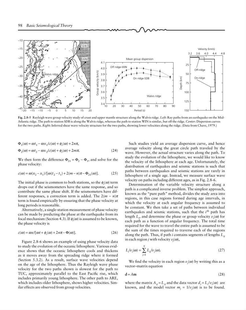
Fig. 2.8-5 Rayleigh wave group velocity study of crust and upper mantle structure along the Walvis ridge. Left: Ray paths from an earthquake on the MidAtlantic ridge. The path to station SDB is along the Walvis ridge, whereas the path to station WIN is similar, but off the ridge. Center: Dispersion curves
for the two paths. Right: Inferred shear wave velocity structure for the two paths, showing lower velocities along the ridge. (Data from Chave, 1979.)
Φ 1 (ω) = ω t 1 − ω x 1 /c(ω) + φ i (ω) + 2nπ,
Φ 2 (ω) = ω t 2 − ω x 2 /c(ω) + φ i (ω) + 2mπ.
(24)
We then form the difference Φ 21 = Φ 2 − Φ 1 , and solve for the
phase velocity:
c(ω) = ω (x 2 − x 1 )/[ω (t 2 − t 1 ) + 2(m − n)π − Φ 21 (ω)].
(25)
The initial phase is common to both stations, so the φ i (ω) term
drops out if the seismometers have the same response, and so
contribute the same phase shift. If the seismometers have different responses, a correction term is added. The 2(m − n)π
term is found empirically by ensuring that the phase velocity at
long periods is reasonable.
Alternatively, a single-station measurement of phase velocity
can be made by predicting the phase at the earthquake from its
focal mechanism (Section 4.3). If φ i (ω) is assumed to be known,
the phase velocity is
c(ω) = ωx/[ω t + φ i (ω) + 2nπ − Φ(ω)].
(26)
Figure 2.8-6 shows an example of using phase velocity data
to study the evolution of the oceanic lithosphere. Various evidence shows that the oceanic lithosphere cools and thickens
as it moves away from the spreading ridge where it formed
(Section 5.3.2). As a result, surface wave velocities depend
on the age of the lithosphere. Thus the Rayleigh wave phase
velocity for the two paths shown is slowest for the path to
TUC, approximately parallel to the East Pacific rise, which
includes primarily young lithosphere. The other path to ARE,
which includes older lithosphere, shows higher velocities. Similar effects are observed from group velocities.
Such studies yield an average dispersion curve, and hence
average velocity along the great circle path traveled by the
wave. However, the actual structure varies along the path. To
study the evolution of the lithosphere, we would like to know
the velocity of the lithosphere at each age. Unfortunately, the
distribution of earthquakes and seismic stations is such that
paths between earthquakes and seismic stations are rarely in
lithosphere of a single age. Instead, we measure surface wave
velocity on paths including different ages, as in Fig. 2.8-6.
Determination of the variable velocity structure along a
path is a complicated inverse problem. The simplest approach,
known as the “pure path” method, divides the study area into
regions, in this case regions formed during age intervals, in
which the velocity at each angular frequency is assumed to
be constant. We then take a set of paths between individual
earthquakes and seismic stations, such that the i th path has
length L i , and determine the phase or group velocity v i (ω) for
each path as a function of angular frequency. The total time
required for the wave to travel the entire path is assumed to be
the sum of the times required to traverse each of the regions
along the path. Thus, if path i contains segments of lengths L ij
in each region j with velocity v j (ω),
L v
L v
i i
ij j
j
n
/ ( )
/ ( ).
ω
ω
=
=
∑
1
(27)
We find the velocity in each region v j (ω) by writing this as a
vector–matrix equation
d = Am
(28)
where the matrix A ij = L ij and the data vector d i = L i /v i (ω) are
known, and the model vector m j = 1/v j (ω) is to be found.
−10
−20 −15 −10
−5
0
5
10
15
20
4.8
25
50
75
100
125
150
4.4
4.0
3.6
3.2
Velocity (km/s)
Off-ridge
On-ridge
Depth (km)
Walvis ridge
SDB
Period (s)
90
4.1
4.0
3.9
3.8
3.7
3.6
3.5
3.4
80
70
60
50
40
30
20
10
Walvis ridge
Off ridge-WIN
On ridge-SDB
Mean group dispersion
Group velocity (km/s)
−15
−20
−25
−30
−35
−40
−45
WIN
Fig. 2.8-5 Rayleigh wave group velocity study of crust and upper mantle structure along the Walvis ridge. Left: Ray paths from an earthquake on the MidAtlantic ridge. The path to station SDB is along the Walvis ridge, whereas the path to station WIN is similar, but off the ridge. Center: Dispersion curves
for the two paths. Right: Inferred shear wave velocity structure for the two paths, showing lower velocities along the ridge. (Data from Chave, 1979.)
Φ 1 (ω) = ω t 1 − ω x 1 /c(ω) + φ i (ω) + 2nπ,
Φ 2 (ω) = ω t 2 − ω x 2 /c(ω) + φ i (ω) + 2mπ.
(24)
We then form the difference Φ 21 = Φ 2 − Φ 1 , and solve for the
phase velocity:
c(ω) = ω (x 2 − x 1 )/[ω (t 2 − t 1 ) + 2(m − n)π − Φ 21 (ω)].
(25)
The initial phase is common to both stations, so the φ i (ω) term
drops out if the seismometers have the same response, and so
contribute the same phase shift. If the seismometers have different responses, a correction term is added. The 2(m − n)π
term is found empirically by ensuring that the phase velocity at
long periods is reasonable.
Alternatively, a single-station measurement of phase velocity
can be made by predicting the phase at the earthquake from its
focal mechanism (Section 4.3). If φ i (ω) is assumed to be known,
the phase velocity is
c(ω) = ωx/[ω t + φ i (ω) + 2nπ − Φ(ω)].
(26)
Figure 2.8-6 shows an example of using phase velocity data
to study the evolution of the oceanic lithosphere. Various evidence shows that the oceanic lithosphere cools and thickens
as it moves away from the spreading ridge where it formed
(Section 5.3.2). As a result, surface wave velocities depend
on the age of the lithosphere. Thus the Rayleigh wave phase
velocity for the two paths shown is slowest for the path to
TUC, approximately parallel to the East Pacific rise, which
includes primarily young lithosphere. The other path to ARE,
which includes older lithosphere, shows higher velocities. Similar effects are observed from group velocities.
Such studies yield an average dispersion curve, and hence
average velocity along the great circle path traveled by the
wave. However, the actual structure varies along the path. To
study the evolution of the lithosphere, we would like to know
the velocity of the lithosphere at each age. Unfortunately, the
distribution of earthquakes and seismic stations is such that
paths between earthquakes and seismic stations are rarely in
lithosphere of a single age. Instead, we measure surface wave
velocity on paths including different ages, as in Fig. 2.8-6.
Determination of the variable velocity structure along a
path is a complicated inverse problem. The simplest approach,
known as the “pure path” method, divides the study area into
regions, in this case regions formed during age intervals, in
which the velocity at each angular frequency is assumed to
be constant. We then take a set of paths between individual
earthquakes and seismic stations, such that the i th path has
length L i , and determine the phase or group velocity v i (ω) for
each path as a function of angular frequency. The total time
required for the wave to travel the entire path is assumed to be
the sum of the times required to traverse each of the regions
along the path. Thus, if path i contains segments of lengths L ij
in each region j with velocity v j (ω),
L v
L v
i i
ij j
j
n
/ ( )
/ ( ).
ω
ω
=
=
∑
1
(27)
We find the velocity in each region v j (ω) by writing this as a
vector–matrix equation
d = Am
(28)
where the matrix A ij = L ij and the data vector d i = L i /v i (ω) are
known, and the model vector m j = 1/v j (ω) is to be found.