

4.5
Group velocity (km/s)
4.0
3.5
3.0
1 /10 unit
unit amp.
Transverse
Unfiltered
2:10
T = 14.5 s
19.0
28.0
51.0
109.0
2:15
+
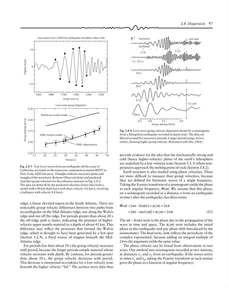
Fig. 2.8-4 Love wave group velocity dispersion shown by a seismogram
from a Mongolian earthquake recorded in Japan (top). The data are
filtered around five successive periods. Longer period energy arrives
earlier, showing higher group velocity. (Kanamori and Abe, 1968.)
Group velocity (km/s)
4.25
4.00
3.75
3.50
3.25
15
Period (s)
50
20
25
30
35
40
45
Digital counts
10
0
−10
1020
Origin time (s)
1080
1140
1200
Love wave group dispersion
Love waves from California earthquake recorded in New York
Reference crustal model
RSNY inverse model
RSNY observations
1320
1260
Fig. 2.8-3 Top: Love waves from an earthquake off the coast of
California, recorded on the transverse component at station RSNY in
New York, 4200 km away. Triangles indicate successive peaks and
troughs of the waveform. Bottom: Observed (dots) and predicted
(top line) group velocities for the reference structure in Fig. 2.8-2.
The data are better fit by the predicted velocities (lower line) from a
model with a 40 km-thick layer with shear velocity 3.6 km /s, overlying
a halfspace with velocity 4.4 km/s.
2.8 Dispersion 97
ridge, a linear elevated region in the South Atlantic. There are
noticeable group velocity differences between two paths from
an earthquake on the Mid-Atlantic ridge, one along the Walvis
ridge and one off the ridge. For periods greater than about 20 s
the off-ridge path is faster, indicating the presence of highervelocity upper mantle material to a depth of about 45 km. This
difference may reflect the processes that formed the Walvis
ridge, which is thought to have been generated by a hot spot
(Section 5.2.4), a fixed source of magma beneath the MidAtlantic ridge.
For periods less than about 50 s the group velocity increases
with period, because the longer periods sample material whose
velocity increases with depth. By contrast, for periods greater
than about 50 s, the group velocity decreases with period.
This decrease is interpreted as evidence for a low-velocity zone
beneath the higher velocity “lid.” The surface wave data thus
provide evidence for the idea that the mechanically strong and
cold (hence higher-velocity) plates of the earth’s lithosphere
are underlain by a low-velocity zone (Section 3.5.3) where temperatures approach the melting point of rock (Section 3.8.2).
Earth structure is also studied using phase velocities. These
are more difficult to measure than group velocities, because
they are defined for harmonic waves of a single frequency.
Taking the Fourier transform of a seismogram yields the phase
at each angular frequency, Φ(ω). We assume that this phase,
on a seismogram recorded at a distance x from an earthquake
at time t after the earthquake, has three terms
Φ(ω) = [ωt − k(ω)x] + φ i (ω) + 2nπ
= [ωt − ωx/c(ω)] + φ i (ω) + 2nπ.
(23)
The ωt − k(ω)x term is the phase due to the propagation of the
wave in time and space. The φ i (ω) term includes the initial
phase at the earthquake and any phase shift introduced by the
seismometer. The final term, 2nπ, reflects the periodicity of the
complex exponential, because adding an integral multiple of
2π to the argument yields the same value.
The phase velocity can be found from observations in two
ways. One method uses seismograms recorded at two stations,
at distances x 1 and x 2 from an earthquake. If the waves arrive
at times t 1 and t 2 , taking the Fourier transform at each station
gives the phase as a function of angular frequency:
Group velocity (km/s)
4.0
3.5
3.0
1 /10 unit
unit amp.
Transverse
Unfiltered
2:10
T = 14.5 s
19.0
28.0
51.0
109.0
2:15
+
Fig. 2.8-4 Love wave group velocity dispersion shown by a seismogram
from a Mongolian earthquake recorded in Japan (top). The data are
filtered around five successive periods. Longer period energy arrives
earlier, showing higher group velocity. (Kanamori and Abe, 1968.)
Group velocity (km/s)
4.25
4.00
3.75
3.50
3.25
15
Period (s)
50
20
25
30
35
40
45
Digital counts
10
0
−10
1020
Origin time (s)
1080
1140
1200
Love wave group dispersion
Love waves from California earthquake recorded in New York
Reference crustal model
RSNY inverse model
RSNY observations
1320
1260
Fig. 2.8-3 Top: Love waves from an earthquake off the coast of
California, recorded on the transverse component at station RSNY in
New York, 4200 km away. Triangles indicate successive peaks and
troughs of the waveform. Bottom: Observed (dots) and predicted
(top line) group velocities for the reference structure in Fig. 2.8-2.
The data are better fit by the predicted velocities (lower line) from a
model with a 40 km-thick layer with shear velocity 3.6 km /s, overlying
a halfspace with velocity 4.4 km/s.
2.8 Dispersion 97
ridge, a linear elevated region in the South Atlantic. There are
noticeable group velocity differences between two paths from
an earthquake on the Mid-Atlantic ridge, one along the Walvis
ridge and one off the ridge. For periods greater than about 20 s
the off-ridge path is faster, indicating the presence of highervelocity upper mantle material to a depth of about 45 km. This
difference may reflect the processes that formed the Walvis
ridge, which is thought to have been generated by a hot spot
(Section 5.2.4), a fixed source of magma beneath the MidAtlantic ridge.
For periods less than about 50 s the group velocity increases
with period, because the longer periods sample material whose
velocity increases with depth. By contrast, for periods greater
than about 50 s, the group velocity decreases with period.
This decrease is interpreted as evidence for a low-velocity zone
beneath the higher velocity “lid.” The surface wave data thus
provide evidence for the idea that the mechanically strong and
cold (hence higher-velocity) plates of the earth’s lithosphere
are underlain by a low-velocity zone (Section 3.5.3) where temperatures approach the melting point of rock (Section 3.8.2).
Earth structure is also studied using phase velocities. These
are more difficult to measure than group velocities, because
they are defined for harmonic waves of a single frequency.
Taking the Fourier transform of a seismogram yields the phase
at each angular frequency, Φ(ω). We assume that this phase,
on a seismogram recorded at a distance x from an earthquake
at time t after the earthquake, has three terms
Φ(ω) = [ωt − k(ω)x] + φ i (ω) + 2nπ
= [ωt − ωx/c(ω)] + φ i (ω) + 2nπ.
(23)
The ωt − k(ω)x term is the phase due to the propagation of the
wave in time and space. The φ i (ω) term includes the initial
phase at the earthquake and any phase shift introduced by the
seismometer. The final term, 2nπ, reflects the periodicity of the
complex exponential, because adding an integral multiple of
2π to the argument yields the same value.
The phase velocity can be found from observations in two
ways. One method uses seismograms recorded at two stations,
at distances x 1 and x 2 from an earthquake. If the waves arrive
at times t 1 and t 2 , taking the Fourier transform at each station
gives the phase as a function of angular frequency: