

96 Basic Seismological Theory
0
1 = 3.9 km/s
β
2 = 4.6 km/s
β
1 = 2.8 g/cm
3
ρ
2 = 3.3 g/cm
3
ρ
h = 40 km
Love wave dispersion
50
100
150
c
4.6
4.4
4.2
4.0
3.8
Velocity (km/s)
Period (s)
U
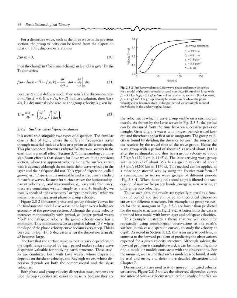
Fig. 2.8-2 Fundamental mode Love wave phase and group velocities
for a model of the continental crust and mantle, a 40 km-thick layer with
β 1 = 3.9 km /s, ρ 1 = 2.8 g/cm 3 underlain by a halfspace with β 2 = 4.6 km /s,
ρ 2 = 3.3 g/cm
3 . The group velocity has a minimum where the phase
velocity curve becomes steep, as longer-period waves sample more of
the velocity in the underlying halfspace.
For a dispersive wave, such as the Love wave in the previous
section, the group velocity can be found from the dispersion
relation. If the dispersion relation is
f(ω, k) = 0,
(20)
then the change in f for a small change in ω and k is given by the
Taylor series,
f(ω + dω, k + dk) = f(ω, k) +
∂
∂
∂
∂
f d
f
k
dk
k
ω
ω
ω
.
+
(21)
Because ω and k define a mode, they satisfy the dispersion relation, f(ω, k) = 0. If ω + dω, k + dk, is also a solution, then f(ω +
dω, k + dk) must also be zero, so the group velocity is given by
U
d
dk
f
k
f
k
.
=
= −
⎛
⎝
⎜
⎞
⎠
⎟
⎛
⎝
⎜
⎞
⎠
⎟
ω
ω
ω
∂
∂
∂
∂
(22)
2.8.3 Surface wave dispersion studies
It is useful to distinguish two types of dispersion. The familiar
case is that of light, where the different frequencies travel
through material such as a lens or a prism at different speeds.
This phenomenon, known as physical dispersion, occurs in the
earth but is a small effect (Section 3.7). In seismology, a more
significant effect is that shown for Love waves in the previous
section, where the apparent velocity along the surface varied
with frequency although the intrinsic shear wave velocity in the
layer and the halfspace did not. This type of dispersion, called
geometrical dispersion, is noticeable and is frequently studied
for surface waves. Because for surface waves the horizontal apparent velocity, c x , and wavenumber, k x , vary with frequency,
these are sometimes written simply as c and k. Similarly, we
usually speak of “phase velocity” or “group velocity” when we
mean horizontal apparent phase or group velocity.
Figure 2.8-2 illustrates phase and group velocity curves for
the fundamental mode Love wave in the layer over a halfspace
geometry of the previous section. Although the phase velocity
increases monotonically with period, as longer period waves
“feel” the halfspace velocity, the group velocity curve has a
minimum. This minimum occurs at a period (about 15 s) where
the slope of the phase velocity curve becomes very steep. This is
because, by Eqn 19, U decreases when the dispersion term dc/
dλ becomes large.
The fact that the surface wave velocities vary depending on
the depth range sampled by each period makes surface wave
dispersion valuable for studying earth structure. These studies are conducted both with Love waves, whose dispersion
depends on the shear velocity, and Rayleigh waves, whose dispersion depends on both the compressional and the shear
velocities.
Both phase and group velocity dispersion measurements are
used. Group velocities are easier to measure because they are
the velocities at which a wave group visible on a seismogram
travels. As shown by the Love waves in Fig. 2.8-3, the period
can be measured from the time between successive peaks or
troughs. Generally, the waves with longest periods travel fastest, and therefore appear first on seismograms. The group velocity is found by dividing the distance between the source and
the receiver by the travel time of the wave group. Hence the
wave group with a period of about 45 s arrived about 1145 s
after the earthquake, and thus has a group velocity of about
3.7 km/s (4200 km in 1145 s). The later-arriving wave group
with a period of about 35 s has a group velocity of about
3.6 km/s (4200 km in 1170 s). This method can be applied in
a more sophisticated way by using the Fourier transform of
a seismogram to isolate wave groups of different periods
(Fig. 2.8-4). When the original record (top) is filtered at a succession of narrow frequency bands, energy is seen arriving at
different group velocities.
To use such data, the results are typically plotted as a function of period and are compared to theoretical dispersion
curves for different structures. For example, the group velocities for the seismogram in Fig. 2.8-3 are lower than predicted
for the simple structure in Fig. 2.8-2. A better fit to the data is
obtained for a model with lower layer and halfspace velocities.
This example illustrates a theme that we will encounter
repeatedly: using seismological observations at the earth’s
surface (in this case dispersion curves), to study the velocity at
depth. As noted in Section 1.1.2, this is an inverse problem, in
contrast to the forward problem of predicting the observations
expected for a given velocity structure. Although solving the
forward problem is straightforward, it can be more difficult to
find a model or models consistent with the observations. For
the moment, we assume that such a model can be found, if only
by trial and error, and defer more detailed discussion until
Chapter 7.
Dispersion data are used to study more complicated velocity
structures. Figure 2.8-5 shows the observed dispersion curves
and inferred S-wave velocity structure for a study of the Walvis
0
1 = 3.9 km/s
β
2 = 4.6 km/s
β
1 = 2.8 g/cm
3
ρ
2 = 3.3 g/cm
3
ρ
h = 40 km
Love wave dispersion
50
100
150
c
4.6
4.4
4.2
4.0
3.8
Velocity (km/s)
Period (s)
U
Fig. 2.8-2 Fundamental mode Love wave phase and group velocities
for a model of the continental crust and mantle, a 40 km-thick layer with
β 1 = 3.9 km /s, ρ 1 = 2.8 g/cm 3 underlain by a halfspace with β 2 = 4.6 km /s,
ρ 2 = 3.3 g/cm
3 . The group velocity has a minimum where the phase
velocity curve becomes steep, as longer-period waves sample more of
the velocity in the underlying halfspace.
For a dispersive wave, such as the Love wave in the previous
section, the group velocity can be found from the dispersion
relation. If the dispersion relation is
f(ω, k) = 0,
(20)
then the change in f for a small change in ω and k is given by the
Taylor series,
f(ω + dω, k + dk) = f(ω, k) +
∂
∂
∂
∂
f d
f
k
dk
k
ω
ω
ω
.
+
(21)
Because ω and k define a mode, they satisfy the dispersion relation, f(ω, k) = 0. If ω + dω, k + dk, is also a solution, then f(ω +
dω, k + dk) must also be zero, so the group velocity is given by
U
d
dk
f
k
f
k
.
=
= −
⎛
⎝
⎜
⎞
⎠
⎟
⎛
⎝
⎜
⎞
⎠
⎟
ω
ω
ω
∂
∂
∂
∂
(22)
2.8.3 Surface wave dispersion studies
It is useful to distinguish two types of dispersion. The familiar
case is that of light, where the different frequencies travel
through material such as a lens or a prism at different speeds.
This phenomenon, known as physical dispersion, occurs in the
earth but is a small effect (Section 3.7). In seismology, a more
significant effect is that shown for Love waves in the previous
section, where the apparent velocity along the surface varied
with frequency although the intrinsic shear wave velocity in the
layer and the halfspace did not. This type of dispersion, called
geometrical dispersion, is noticeable and is frequently studied
for surface waves. Because for surface waves the horizontal apparent velocity, c x , and wavenumber, k x , vary with frequency,
these are sometimes written simply as c and k. Similarly, we
usually speak of “phase velocity” or “group velocity” when we
mean horizontal apparent phase or group velocity.
Figure 2.8-2 illustrates phase and group velocity curves for
the fundamental mode Love wave in the layer over a halfspace
geometry of the previous section. Although the phase velocity
increases monotonically with period, as longer period waves
“feel” the halfspace velocity, the group velocity curve has a
minimum. This minimum occurs at a period (about 15 s) where
the slope of the phase velocity curve becomes very steep. This is
because, by Eqn 19, U decreases when the dispersion term dc/
dλ becomes large.
The fact that the surface wave velocities vary depending on
the depth range sampled by each period makes surface wave
dispersion valuable for studying earth structure. These studies are conducted both with Love waves, whose dispersion
depends on the shear velocity, and Rayleigh waves, whose dispersion depends on both the compressional and the shear
velocities.
Both phase and group velocity dispersion measurements are
used. Group velocities are easier to measure because they are
the velocities at which a wave group visible on a seismogram
travels. As shown by the Love waves in Fig. 2.8-3, the period
can be measured from the time between successive peaks or
troughs. Generally, the waves with longest periods travel fastest, and therefore appear first on seismograms. The group velocity is found by dividing the distance between the source and
the receiver by the travel time of the wave group. Hence the
wave group with a period of about 45 s arrived about 1145 s
after the earthquake, and thus has a group velocity of about
3.7 km/s (4200 km in 1145 s). The later-arriving wave group
with a period of about 35 s has a group velocity of about
3.6 km/s (4200 km in 1170 s). This method can be applied in
a more sophisticated way by using the Fourier transform of
a seismogram to isolate wave groups of different periods
(Fig. 2.8-4). When the original record (top) is filtered at a succession of narrow frequency bands, energy is seen arriving at
different group velocities.
To use such data, the results are typically plotted as a function of period and are compared to theoretical dispersion
curves for different structures. For example, the group velocities for the seismogram in Fig. 2.8-3 are lower than predicted
for the simple structure in Fig. 2.8-2. A better fit to the data is
obtained for a model with lower layer and halfspace velocities.
This example illustrates a theme that we will encounter
repeatedly: using seismological observations at the earth’s
surface (in this case dispersion curves), to study the velocity at
depth. As noted in Section 1.1.2, this is an inverse problem, in
contrast to the forward problem of predicting the observations
expected for a given velocity structure. Although solving the
forward problem is straightforward, it can be more difficult to
find a model or models consistent with the observations. For
the moment, we assume that such a model can be found, if only
by trial and error, and defer more detailed discussion until
Chapter 7.
Dispersion data are used to study more complicated velocity
structures. Figure 2.8-5 shows the observed dispersion curves
and inferred S-wave velocity structure for a study of the Walvis