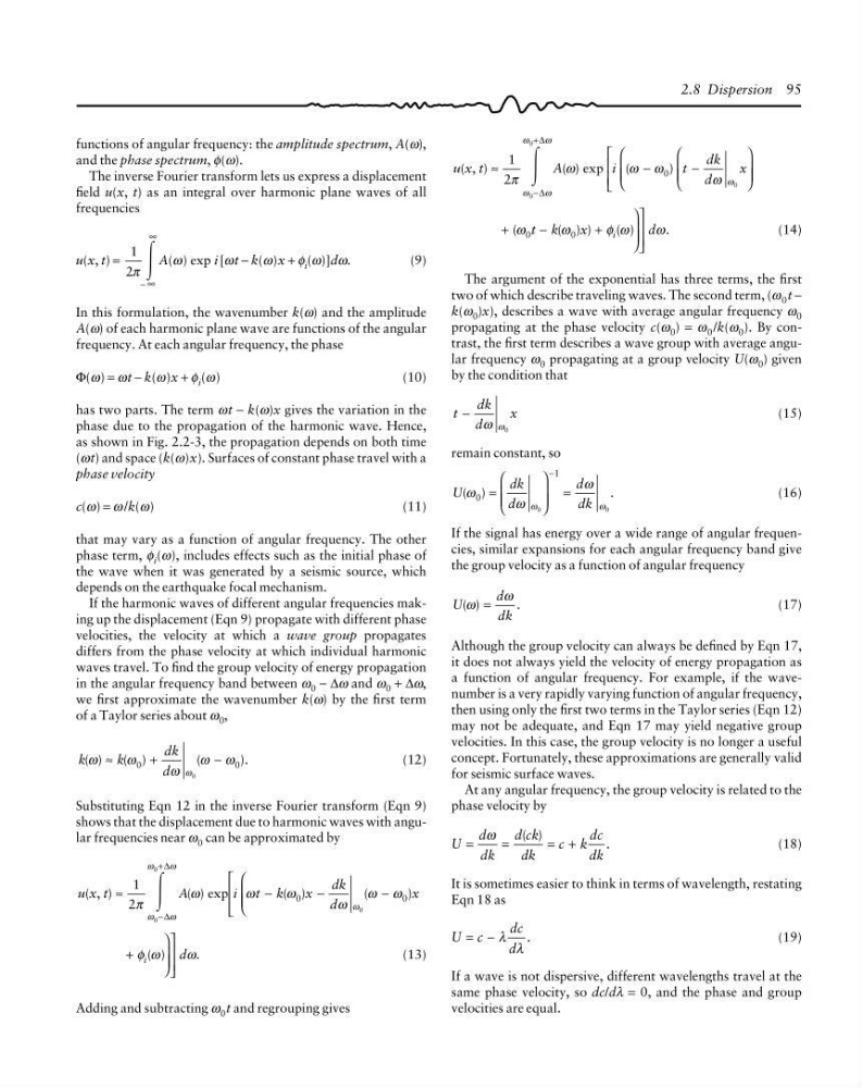
functions of angular frequency: the amplitude spectrum, A(ω),
and the phase spectrum, φ(ω).
The inverse Fourier transform lets us express a displacement
field u(x, t) as an integral over harmonic plane waves of all
frequencies
u(x, t) =
1
2π Ύ
− ∞
∞
A(ω) exp i [ωt − k(ω)x + φ i (ω)]dω.
(9)
In this formulation, the wavenumber k(ω) and the amplitude
A(ω) of each harmonic plane wave are functions of the angular
frequency. At each angular frequency, the phase
Φ(ω) = ωt − k(ω)x + φ i (ω)
(10)
has two parts. The term ωt − k(ω)x gives the variation in the
phase due to the propagation of the harmonic wave. Hence,
as shown in Fig. 2.2-3, the propagation depends on both time
(ωt) and space (k(ω)x). Surfaces of constant phase travel with a
phase velocity
c(ω) = ω /k(ω)
(11)
that may vary as a function of angular frequency. The other
phase term, φ i (ω), includes effects such as the initial phase of
the wave when it was generated by a seismic source, which
depends on the earthquake focal mechanism.
If the harmonic waves of different angular frequencies making up the displacement (Eqn 9) propagate with different phase
velocities, the velocity at which a wave group propagates
differs from the phase velocity at which individual harmonic
waves travel. To find the group velocity of energy propagation
in the angular frequency band between ω 0 − ∆ω and ω 0 + ∆ω,
we first approximate the wavenumber k(ω) by the first term
of a Taylor series about ω 0 ,
k
k
dk
d
( )
( )
(
).
ω
ω
ω
ω ω
ω
≈
+
−
0
0
0
(12)
Substituting Eqn 12 in the inverse Fourier transform (Eqn 9)
shows that the displacement due to harmonic waves with angular frequencies near ω 0 can be approximated by
u x t
A
i t k
x
dk
d
x
( , )
( ) exp
( )
(
)
≈
−
−
−
⎛
⎝
⎜ ⎜
⎡
⎣
⎢
⎢
−
+
1
2
0
0
0
0
0
π
ω
ω
ω
ω
ω ω
ω
ω
ω
ω
ω
Ύ
∆
∆
d
i ( )
.
+
⎞
⎠
⎟ ⎟
⎤
⎦
⎥
⎥
φ ω
ω
(13)
Adding and subtracting ω 0 t and regrouping gives
2.8 Dispersion 95
u x t
A
i
t
dk
d
x
( , )
( ) exp
(
)
≈
−
−
⎛
⎝
⎜ ⎜
⎞
⎠
⎟ ⎟
⎛
⎝
⎜ ⎜
⎡
⎣
⎢
⎢
−
+
1
2
0
0
0
0
π
ω
ω ω
ω
ω
ω
ω
ω
ω
Ύ
∆
∆
t k
x
d
i
(
( ) )
( )
.
+
−
+
⎞
⎠
⎟ ⎟
⎤
⎦
⎥
⎥
0
0
ω
ω
φ ω
ω
(14)
The argument of the exponential has three terms, the first
two of which describe traveling waves. The second term, (ω 0 t −
k(ω 0 )x), describes a wave with average angular frequency ω 0
propagating at the phase velocity c(ω 0 ) = ω 0 /k(ω 0 ). By contrast, the first term describes a wave group with average angular frequency ω 0 propagating at a group velocity U(ω 0 ) given
by the condition that
t
dk
d
x
− ω ω 0
(15)
remain constant, so
U
dk
d
d
dk
( )
.
ω
ω
ω
ω
ω
0
1
0
0
=
⎛
⎝
⎜ ⎜
⎞
⎠
⎟ ⎟
=
−
(16)
If the signal has energy over a wide range of angular frequencies, similar expansions for each angular frequency band give
the group velocity as a function of angular frequency
U
d
dk
( )
.
ω
ω
=
(17)
Although the group velocity can always be defined by Eqn 17,
it does not always yield the velocity of energy propagation as
a function of angular frequency. For example, if the wavenumber is a very rapidly varying function of angular frequency,
then using only the first two terms in the Taylor series (Eqn 12)
may not be adequate, and Eqn 17 may yield negative group
velocities. In this case, the group velocity is no longer a useful
concept. Fortunately, these approximations are generally valid
for seismic surface waves.
At any angular frequency, the group velocity is related to the
phase velocity by
U
d
dk
d ck
dk
c k
dc
dk
( )
.
=
=
= +
ω
(18)
It is sometimes easier to think in terms of wavelength, restating
Eqn 18 as
U c
dc
d
.
= − λ λ
(19)
If a wave is not dispersive, different wavelengths travel at the
same phase velocity, so dc/dλ = 0, and the phase and group
velocities are equal.