

94 Basic Seismological Theory
ω 1 = ω + δω, ω 2 = ω − δω, ω >> δω,
k 1 = k + δk, k 2 = k − δk, k >> δk.
(2)
Using this substitution, we add the two cosines and simplify,
yielding
u(x, t) = cos (ωt + δωt − kx − δkx)
+ cos (ωt − δωt − kx + δkx)
= 2 cos (ωt − kx) cos (δωt − δkx).
(3)
Thus the sum of the two harmonic waves is a product of two
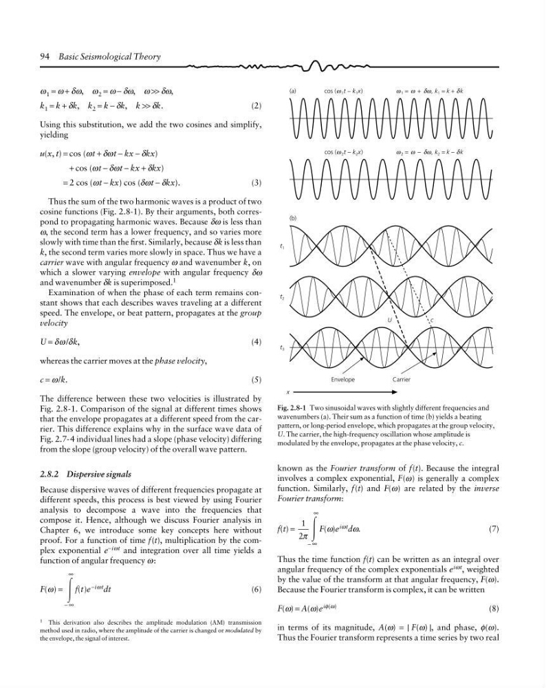
cosine functions (Fig. 2.8-1). By their arguments, both correspond to propagating harmonic waves. Because δω is less than
ω, the second term has a lower frequency, and so varies more
slowly with time than the first. Similarly, because δk is less than
k, the second term varies more slowly in space. Thus we have a
carrier wave with angular frequency ω and wavenumber k, on
which a slower varying envelope with angular frequency δω
and wavenumber δk is superimposed. 1
Examination of when the phase of each term remains constant shows that each describes waves traveling at a different
speed. The envelope, or beat pattern, propagates at the group
velocity
U = δω /δk,
(4)
whereas the carrier moves at the phase velocity,
c = ω /k.
(5)
The difference between these two velocities is illustrated by
Fig. 2.8-1. Comparison of the signal at different times shows
that the envelope propagates at a different speed from the carrier. This difference explains why in the surface wave data of
Fig. 2.7-4 individual lines had a slope (phase velocity) differing
from the slope (group velocity) of the overall wave pattern.
2.8.2 Dispersive signals
Because dispersive waves of different frequencies propagate at
different speeds, this process is best viewed by using Fourier
analysis to decompose a wave into the frequencies that
compose it. Hence, although we discuss Fourier analysis in
Chapter 6, we introduce some key concepts here without
proof. For a function of time f(t), multiplication by the complex exponential e −iωt and integration over all time yields a
function of angular frequency ω :
F(ω) =
Ύ
− ∞
∞
f(t)e
−iω t
dt
(6)
1 This derivation also describes the amplitude modulation (AM) transmission
method used in radio, where the amplitude of the carrier is changed or modulated by
the envelope, the signal of interest.
(a)
cos ( 1 t − k 1 x)
ω
1 =
+
,
ω
ω δω k 1 = k + k
δ
cos ( 2 t − k 2 x)
ω
2 =
−
,
ω
ω δω k 2 = k − k
δ
(b)
t 1
t 2
t 3
x
Envelope
Carrier
U
c
Fig. 2.8-1 Two sinusoidal waves with slightly different frequencies and
wavenumbers (a). Their sum as a function of time (b) yields a beating
pattern, or long-period envelope, which propagates at the group velocity,
U. The carrier, the high-frequency oscillation whose amplitude is
modulated by the envelope, propagates at the phase velocity, c.
known as the Fourier transform of f(t). Because the integral
involves a complex exponential, F(ω) is generally a complex
function. Similarly, f(t) and F(ω) are related by the inverse
Fourier transform:
f(t) =
1
2π Ύ
− ∞
∞
F(ω)e iωt dω.
(7)
Thus the time function f(t) can be written as an integral over
angular frequency of the complex exponentials e iωt , weighted
by the value of the transform at that angular frequency, F(ω).
Because the Fourier transform is complex, it can be written
F(ω) = A(ω)e iφ(ω)
(8)
in terms of its magnitude, A(ω) = | F(ω) |, and phase, φ(ω).
Thus the Fourier transform represents a time series by two real
ω 1 = ω + δω, ω 2 = ω − δω, ω >> δω,
k 1 = k + δk, k 2 = k − δk, k >> δk.
(2)
Using this substitution, we add the two cosines and simplify,
yielding
u(x, t) = cos (ωt + δωt − kx − δkx)
+ cos (ωt − δωt − kx + δkx)
= 2 cos (ωt − kx) cos (δωt − δkx).
(3)
Thus the sum of the two harmonic waves is a product of two
cosine functions (Fig. 2.8-1). By their arguments, both correspond to propagating harmonic waves. Because δω is less than
ω, the second term has a lower frequency, and so varies more
slowly with time than the first. Similarly, because δk is less than
k, the second term varies more slowly in space. Thus we have a
carrier wave with angular frequency ω and wavenumber k, on
which a slower varying envelope with angular frequency δω
and wavenumber δk is superimposed. 1
Examination of when the phase of each term remains constant shows that each describes waves traveling at a different
speed. The envelope, or beat pattern, propagates at the group
velocity
U = δω /δk,
(4)
whereas the carrier moves at the phase velocity,
c = ω /k.
(5)
The difference between these two velocities is illustrated by
Fig. 2.8-1. Comparison of the signal at different times shows
that the envelope propagates at a different speed from the carrier. This difference explains why in the surface wave data of
Fig. 2.7-4 individual lines had a slope (phase velocity) differing
from the slope (group velocity) of the overall wave pattern.
2.8.2 Dispersive signals
Because dispersive waves of different frequencies propagate at
different speeds, this process is best viewed by using Fourier
analysis to decompose a wave into the frequencies that
compose it. Hence, although we discuss Fourier analysis in
Chapter 6, we introduce some key concepts here without
proof. For a function of time f(t), multiplication by the complex exponential e −iωt and integration over all time yields a
function of angular frequency ω :
F(ω) =
Ύ
− ∞
∞
f(t)e
−iω t
dt
(6)
1 This derivation also describes the amplitude modulation (AM) transmission
method used in radio, where the amplitude of the carrier is changed or modulated by
the envelope, the signal of interest.
(a)
cos ( 1 t − k 1 x)
ω
1 =
+
,
ω
ω δω k 1 = k + k
δ
cos ( 2 t − k 2 x)
ω
2 =
−
,
ω
ω δω k 2 = k − k
δ
(b)
t 1
t 2
t 3
x
Envelope
Carrier
U
c
Fig. 2.8-1 Two sinusoidal waves with slightly different frequencies and
wavenumbers (a). Their sum as a function of time (b) yields a beating
pattern, or long-period envelope, which propagates at the group velocity,
U. The carrier, the high-frequency oscillation whose amplitude is
modulated by the envelope, propagates at the phase velocity, c.
known as the Fourier transform of f(t). Because the integral
involves a complex exponential, F(ω) is generally a complex
function. Similarly, f(t) and F(ω) are related by the inverse
Fourier transform:
f(t) =
1
2π Ύ
− ∞
∞
F(ω)e iωt dω.
(7)
Thus the time function f(t) can be written as an integral over
angular frequency of the complex exponentials e iωt , weighted
by the value of the transform at that angular frequency, F(ω).
Because the Fourier transform is complex, it can be written
F(ω) = A(ω)e iφ(ω)
(8)
in terms of its magnitude, A(ω) = | F(ω) |, and phase, φ(ω).
Thus the Fourier transform represents a time series by two real