

1 = 3.9 km/s
β
2 = 4.6 km/s
β
1 = 2.8 g/cm
3
ρ
2 = 3.3 g/cm
3
ρ
h = 40 km
n = 0
n = 1
n = 2
0
50
100
150
200
250
Depth (km)
0
100
Distance (km)
Period
5 s
n = 0
n = 1
Period
10 s
n = 0
Period
30 s
Love wave displacement with depth
n = 2, x = 22, c x = 4.55
λ
5 s
n = 1, x = 20, c x = 4.13
λ
n = 0, x = 19, c x = 3.92
λ
n = 1, x = 45, c x = 4.55
λ
10 s
n = 0, x = 39, c x = 3.98
λ
n = 0, x = 129, c x = 4.30
λ
30 s
Love wave surface displacement
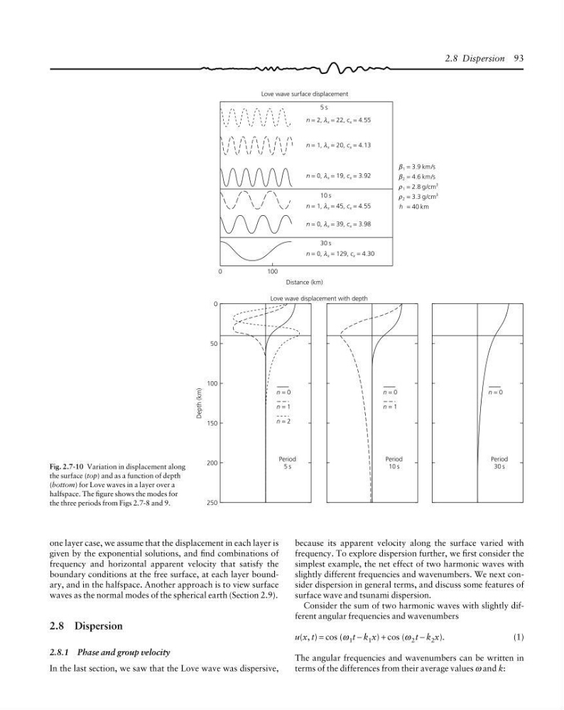
Fig. 2.7-10 Variation in displacement along
the surface (top) and as a function of depth
(bottom) for Love waves in a layer over a
halfspace. The figure shows the modes for
the three periods from Figs 2.7-8 and 9.
2.8 Dispersion 93
because its apparent velocity along the surface varied with
frequency. To explore dispersion further, we first consider the
simplest example, the net effect of two harmonic waves with
slightly different frequencies and wavenumbers. We next consider dispersion in general terms, and discuss some features of
surface wave and tsunami dispersion.
Consider the sum of two harmonic waves with slightly different angular frequencies and wavenumbers
u(x, t) = cos (ω 1 t − k 1 x) + cos (ω 2 t − k 2 x).
(1)
The angular frequencies and wavenumbers can be written in
terms of the differences from their average values ω and k:
one layer case, we assume that the displacement in each layer is
given by the exponential solutions, and find combinations of
frequency and horizontal apparent velocity that satisfy the
boundary conditions at the free surface, at each layer boundary, and in the halfspace. Another approach is to view surface
waves as the normal modes of the spherical earth (Section 2.9).
2.8 Dispersion
2.8.1 Phase and group velocity
In the last section, we saw that the Love wave was dispersive,
β
2 = 4.6 km/s
β
1 = 2.8 g/cm
3
ρ
2 = 3.3 g/cm
3
ρ
h = 40 km
n = 0
n = 1
n = 2
0
50
100
150
200
250
Depth (km)
0
100
Distance (km)
Period
5 s
n = 0
n = 1
Period
10 s
n = 0
Period
30 s
Love wave displacement with depth
n = 2, x = 22, c x = 4.55
λ
5 s
n = 1, x = 20, c x = 4.13
λ
n = 0, x = 19, c x = 3.92
λ
n = 1, x = 45, c x = 4.55
λ
10 s
n = 0, x = 39, c x = 3.98
λ
n = 0, x = 129, c x = 4.30
λ
30 s
Love wave surface displacement
Fig. 2.7-10 Variation in displacement along
the surface (top) and as a function of depth
(bottom) for Love waves in a layer over a
halfspace. The figure shows the modes for
the three periods from Figs 2.7-8 and 9.
2.8 Dispersion 93
because its apparent velocity along the surface varied with
frequency. To explore dispersion further, we first consider the
simplest example, the net effect of two harmonic waves with
slightly different frequencies and wavenumbers. We next consider dispersion in general terms, and discuss some features of
surface wave and tsunami dispersion.
Consider the sum of two harmonic waves with slightly different angular frequencies and wavenumbers
u(x, t) = cos (ω 1 t − k 1 x) + cos (ω 2 t − k 2 x).
(1)
The angular frequencies and wavenumbers can be written in
terms of the differences from their average values ω and k:
one layer case, we assume that the displacement in each layer is
given by the exponential solutions, and find combinations of
frequency and horizontal apparent velocity that satisfy the
boundary conditions at the free surface, at each layer boundary, and in the halfspace. Another approach is to view surface
waves as the normal modes of the spherical earth (Section 2.9).
2.8 Dispersion
2.8.1 Phase and group velocity
In the last section, we saw that the Love wave was dispersive,