

92 Basic Seismological Theory
u +
y (x, z, t) = B′ exp (i(ωt − k x x)) exp (−k x r* β 2 z),
(27)
so, by the continuity of displacement at the interface z = h,
B′ = 2B 1 cos (k x r β 1 h)/exp (−k x r* β 2 h).
(28)
Thus, in both the layer and the halfspace, we have a wave
propagating in the x direction, with horizontal wavenumber
k x = 2π /λ x = ω /c x . In the layer, the displacement varies with
depth as cos (k x r β 1 z), and so oscillates. In the halfspace, the displacement decays exponentially with depth as exp (−k x r* β 2 z).
The variation in displacement in the x and z directions is
illustrated in Fig. 2.7-10 for the three periods whose apparent
velocities were found in Fig. 2.7-8. The horizontal variation
is shown in the upper panels. Because the apparent velocity
increases with period (Fig. 2.7-9), the horizontal wavelength
increases with period for a given branch. Thus, for the fundamental mode (n = 0) cases shown, the longest period (30 s)
has the highest apparent velocity and thus the longest horizontal wavelength. At a given period (Fig. 2.7-9), the higher
the mode, the higher the apparent velocity, and thus the longer
the horizontal wavelength. Hence for the three modes shown
for period 5 s, n = 2 has the longest horizontal wavelength.
The variation with depth, known as the mode’s vertical
eigenfunction, is different for each mode. For a given branch,
the depth of penetration in the halfspace increases with period,
so, of the fundamental mode periods shown, the longest (30 s)
“sees” deepest into the higher velocity halfspace, and thus has
the highest apparent velocity. Conversely, the shortest period
modes on a given branch penetrate to the shallowest depth, and
thus have the lowest apparent velocity. At a given period, the
higher modes oscillate more rapidly with depth in the layer,
and so change sign more frequently. In the halfspace, however,
the higher modes decay more slowly and penetrate deeper. The
eigenfunction for a mode with order n has n zero crossings, or
nodes, with depth.
The fact that the displacement behaves differently with depth
for various modes and periods makes Love waves dispersive.
In our derivation, the intrinsic shear velocities of the layer
and halfspace do not depend on frequency. Nonetheless, the
resulting apparent velocity along the free surface depends on
frequency. This dispersion results from the fact that Love waves
of different periods have different displacements with depth,
and the intrinsic medium velocity varies with depth. As a result,
surface wave dispersion is valuable for studying earth structure.
By contrast, the halfspace Rayleigh wave does not show this
dispersion. This wave is a “true” surface wave because it can
exist in a homogeneous halfspace due to the interaction of P
and SV waves. By contrast, the Love wave in a layer over a
halfspace exists because the properties of the medium vary with
depth, and so cause interference between SH waves. Dispersive
Love waves and Rayleigh waves also occur in media whose
properties vary with depth in a more complicated way. The dispersion curves for Love and Rayleigh waves in such media can
be calculated by several methods. One approach is to extend
the method used in Section 2.7.3 by treating the medium as a
set of homogeneous layers underlain by a halfspace. As for the
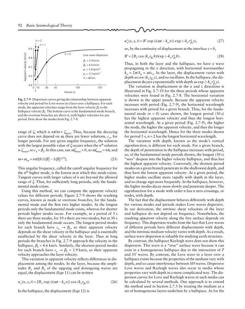
Fig. 2.7-9 Dispersion curves giving the relationship between apparent
velocity and period for Love waves in a layer over a halfspace. For each
mode, the apparent velocities range from the layer velocity β 1 to the
halfspace velocity β 2 . The bottom curve is the fundamental mode branch,
and the overtone branches are above it, with higher velocities for any
period. Dots show the modes from Fig. 2.7-8.
0
1 = 3.9 km/s
β
2 = 4.6 km/s
β
1 = 2.8 g/cm
3
ρ
2 = 3.3 g/cm
3
ρ
h = 40 km
Love wave dispersion
10
50
100
150
n = 0
n = 1
4.6
4.4
4.2
4.0
3.8
Apparent velocity (km/s)
Period (s)
5
30
n = 2
range of ζ, which is nπ/ω < ζ max . Thus, because the decaying
curve does not depend on ω, there are fewer solutions, c x , for
longer periods. For any given angular frequency, the solution
with the largest possible value of ζ occurs when the n th solution
is ζ max , so c x = β 2 . In this case, tan ωζ max = 0, so ωζ max = nπ, and
ω = ω cn = nπ/[h(1/β 2
1 − 1/β 2
2 ) 1/2 ].
(25)
This angular frequency, called the cutoff angular frequency for
the n th higher mode, is the lowest ω at which this mode exists.
Tangent curves with larger values of n are beyond the allowed
range of ζ. Thus, for sufficiently long periods, only the fundamental mode exists.
Using this method, we can compute the apparent velocity
values for different periods. Figure 2.7-9 shows the resulting
curves, known as mode or overtone branches, for the fundamental mode and the first two higher modes. At the longest
periods only the fundamental mode exists, whereas for shorter
periods higher modes occur. For example, at a period of 5 s
there are three modes, for 10 s there are two modes, but at 30 s
only the fundamental mode occurs. The longest-period modes
for each branch have c x → β 2 , so their apparent velocity
depends on the shear velocity in the halfspace and is essentially
unaffected by the shear velocity in the layer. Thus at long
periods the branches in Fig. 2.7-9 approach the velocity in the
halfspace, β 2 = 4.6 km/s. Similarly, the shortest-period modes
for each branch have c x → β 1 = 3.9 km/s, so their apparent
velocity approaches the layer velocity.
This variation in apparent velocity reflects differences in displacement among the modes. In the layer, because the amplitudes B 1 and B 2 of the upgoing and downgoing waves are
equal, the displacement (Eqn 11) can be written
u −
y (x, z, t) = 2B 1 exp (i(ωt − k x x)) cos (k x r β 1 z).
(26)
In the halfspace, the displacement (Eqn 12) is
u +
y (x, z, t) = B′ exp (i(ωt − k x x)) exp (−k x r* β 2 z),
(27)
so, by the continuity of displacement at the interface z = h,
B′ = 2B 1 cos (k x r β 1 h)/exp (−k x r* β 2 h).
(28)
Thus, in both the layer and the halfspace, we have a wave
propagating in the x direction, with horizontal wavenumber
k x = 2π /λ x = ω /c x . In the layer, the displacement varies with
depth as cos (k x r β 1 z), and so oscillates. In the halfspace, the displacement decays exponentially with depth as exp (−k x r* β 2 z).
The variation in displacement in the x and z directions is
illustrated in Fig. 2.7-10 for the three periods whose apparent
velocities were found in Fig. 2.7-8. The horizontal variation
is shown in the upper panels. Because the apparent velocity
increases with period (Fig. 2.7-9), the horizontal wavelength
increases with period for a given branch. Thus, for the fundamental mode (n = 0) cases shown, the longest period (30 s)
has the highest apparent velocity and thus the longest horizontal wavelength. At a given period (Fig. 2.7-9), the higher
the mode, the higher the apparent velocity, and thus the longer
the horizontal wavelength. Hence for the three modes shown
for period 5 s, n = 2 has the longest horizontal wavelength.
The variation with depth, known as the mode’s vertical
eigenfunction, is different for each mode. For a given branch,
the depth of penetration in the halfspace increases with period,
so, of the fundamental mode periods shown, the longest (30 s)
“sees” deepest into the higher velocity halfspace, and thus has
the highest apparent velocity. Conversely, the shortest period
modes on a given branch penetrate to the shallowest depth, and
thus have the lowest apparent velocity. At a given period, the
higher modes oscillate more rapidly with depth in the layer,
and so change sign more frequently. In the halfspace, however,
the higher modes decay more slowly and penetrate deeper. The
eigenfunction for a mode with order n has n zero crossings, or
nodes, with depth.
The fact that the displacement behaves differently with depth
for various modes and periods makes Love waves dispersive.
In our derivation, the intrinsic shear velocities of the layer
and halfspace do not depend on frequency. Nonetheless, the
resulting apparent velocity along the free surface depends on
frequency. This dispersion results from the fact that Love waves
of different periods have different displacements with depth,
and the intrinsic medium velocity varies with depth. As a result,
surface wave dispersion is valuable for studying earth structure.
By contrast, the halfspace Rayleigh wave does not show this
dispersion. This wave is a “true” surface wave because it can
exist in a homogeneous halfspace due to the interaction of P
and SV waves. By contrast, the Love wave in a layer over a
halfspace exists because the properties of the medium vary with
depth, and so cause interference between SH waves. Dispersive
Love waves and Rayleigh waves also occur in media whose
properties vary with depth in a more complicated way. The dispersion curves for Love and Rayleigh waves in such media can
be calculated by several methods. One approach is to extend
the method used in Section 2.7.3 by treating the medium as a
set of homogeneous layers underlain by a halfspace. As for the
Fig. 2.7-9 Dispersion curves giving the relationship between apparent
velocity and period for Love waves in a layer over a halfspace. For each
mode, the apparent velocities range from the layer velocity β 1 to the
halfspace velocity β 2 . The bottom curve is the fundamental mode branch,
and the overtone branches are above it, with higher velocities for any
period. Dots show the modes from Fig. 2.7-8.
0
1 = 3.9 km/s
β
2 = 4.6 km/s
β
1 = 2.8 g/cm
3
ρ
2 = 3.3 g/cm
3
ρ
h = 40 km
Love wave dispersion
10
50
100
150
n = 0
n = 1
4.6
4.4
4.2
4.0
3.8
Apparent velocity (km/s)
Period (s)
5
30
n = 2
range of ζ, which is nπ/ω < ζ max . Thus, because the decaying
curve does not depend on ω, there are fewer solutions, c x , for
longer periods. For any given angular frequency, the solution
with the largest possible value of ζ occurs when the n th solution
is ζ max , so c x = β 2 . In this case, tan ωζ max = 0, so ωζ max = nπ, and
ω = ω cn = nπ/[h(1/β 2
1 − 1/β 2
2 ) 1/2 ].
(25)
This angular frequency, called the cutoff angular frequency for
the n th higher mode, is the lowest ω at which this mode exists.
Tangent curves with larger values of n are beyond the allowed
range of ζ. Thus, for sufficiently long periods, only the fundamental mode exists.
Using this method, we can compute the apparent velocity
values for different periods. Figure 2.7-9 shows the resulting
curves, known as mode or overtone branches, for the fundamental mode and the first two higher modes. At the longest
periods only the fundamental mode exists, whereas for shorter
periods higher modes occur. For example, at a period of 5 s
there are three modes, for 10 s there are two modes, but at 30 s
only the fundamental mode occurs. The longest-period modes
for each branch have c x → β 2 , so their apparent velocity
depends on the shear velocity in the halfspace and is essentially
unaffected by the shear velocity in the layer. Thus at long
periods the branches in Fig. 2.7-9 approach the velocity in the
halfspace, β 2 = 4.6 km/s. Similarly, the shortest-period modes
for each branch have c x → β 1 = 3.9 km/s, so their apparent
velocity approaches the layer velocity.
This variation in apparent velocity reflects differences in displacement among the modes. In the layer, because the amplitudes B 1 and B 2 of the upgoing and downgoing waves are
equal, the displacement (Eqn 11) can be written
u −
y (x, z, t) = 2B 1 exp (i(ωt − k x x)) cos (k x r β 1 z).
(26)
In the halfspace, the displacement (Eqn 12) is