

using cos 2j 1 = cos 2 j 1 − 1. The condition for constructive interference is thus that the total phase change
−2k β 1 h cos j 1 + 2 tan
−1 [(µ 2 r* β 2 )/(µ 1 r β 1 )] = 2nπ,
(20)
or, because tan (nπ) = 0,
tan (k β 1 h cos j 1 ) = tan (k x r β 1 h) = (µ 2 r* β 2 )/(µ 1 r β 1 ).
(21)
Thus the Love wave dispersion relation that we derived from
the boundary conditions can also be viewed as an interference
criterion for post-critically reflected SH waves, corresponding
to propagating waves in the layer and an evanescent wave in
the higher-velocity halfspace.
2.7.4 Love wave dispersion
The dispersion relation (Eqn 21) can be written as a function
of any two of the three related parameters c x , ω, and k x . To
find solutions, we write it in terms of frequency and apparent
velocity as
tan [(ωh/c x )(c 2
x /β 2
1 − 1) 1/2 ] =
−
−
(
/ )
( /
)
.
/
/
µ
β
µ
β
2
2
2
2 1 2
1
2
1
2
12
1
1
c
c
x
x
(22)
Because the tangent function is defined for real values, the
square roots must be real, so the apparent velocity is bounded
by β 1 < c x < β 2 . A graphical solution can be derived by defining a
new variable,
ζ = (h/c x )(c 2
x /β 2
1 − 1) 1/2 ,
(23)
so that over the allowable range of the apparent velocity,
ζ = 0 at c x = β 1 , and ζ max = h(1/β 2
1 − 1/β 2
2 ) 1/2 at c x = β 2 . Hence,
Eqn 22 becomes
tan ( )
(
/ )
.
/
ωξ
µ
β
µ
ξ
=
−
⎛
⎝
⎜
⎞
⎠
⎟
⎛
⎝
⎜
⎞
⎠
⎟
2
2
2
2 1 2
1
1 c
h
c
z
z
(24)
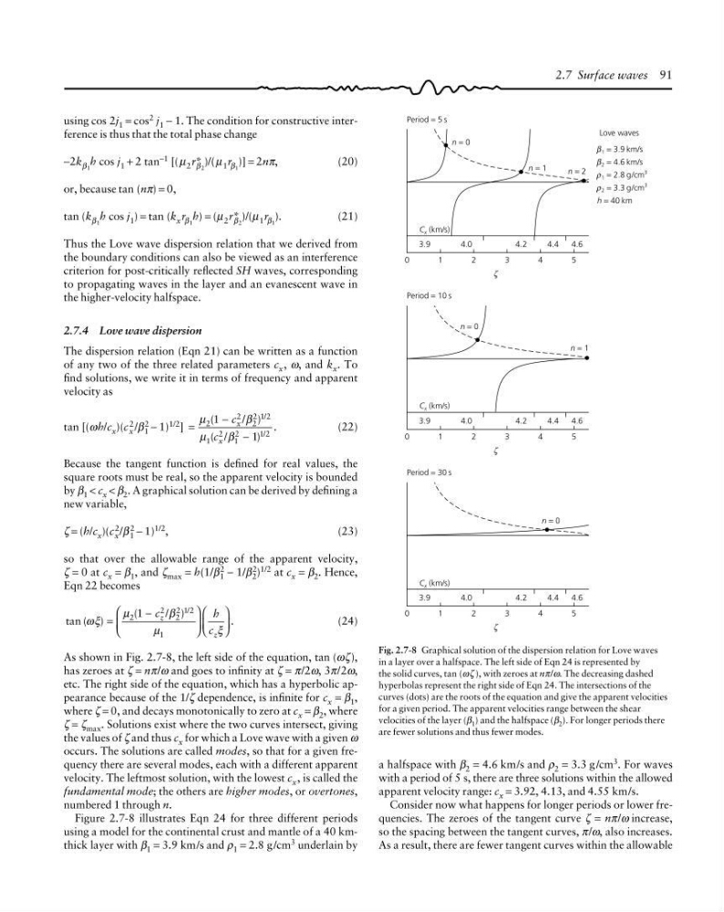
As shown in Fig. 2.7-8, the left side of the equation, tan (ωζ),
has zeroes at ζ = nπ/ω and goes to infinity at ζ = π/2ω, 3π/2ω,
etc. The right side of the equation, which has a hyperbolic appearance because of the 1/ζ dependence, is infinite for c x = β 1 ,
where ζ = 0, and decays monotonically to zero at c x = β 2 , where
ζ = ζ max . Solutions exist where the two curves intersect, giving
the values of ζ and thus c x for which a Love wave with a given ω
occurs. The solutions are called modes, so that for a given frequency there are several modes, each with a different apparent
velocity. The leftmost solution, with the lowest c x , is called the
fundamental mode; the others are higher modes, or overtones,
numbered 1 through n.
Figure 2.7-8 illustrates Eqn 24 for three different periods
using a model for the continental crust and mantle of a 40 kmthick layer with β 1 = 3.9 km/s and ρ 1 = 2.8 g /cm 3 underlain by
Fig. 2.7-8 Graphical solution of the dispersion relation for Love waves
in a layer over a halfspace. The left side of Eqn 24 is represented by
the solid curves, tan (ωζ ), with zeroes at nπ/ω. The decreasing dashed
hyperbolas represent the right side of Eqn 24. The intersections of the
curves (dots) are the roots of the equation and give the apparent velocities
for a given period. The apparent velocities range between the shear
velocities of the layer (β 1 ) and the halfspace (β 2 ). For longer periods there
are fewer solutions and thus fewer modes.
2.7 Surface waves 91
0
ζ
1 = 3.9 km/s
β
2 = 4.6 km/s
β
1 = 2.8 g/cm
3
ρ
2 = 3.3 g/cm
3
ρ
h = 40 km
Love waves
1
2
3
4
5
n = 0
3.9
4.0
4.2
4.4
4.6
0
ζ
1
2
3
4
5
Period = 10 s
3.9
4.0
4.2
4.4
4.6
0
ζ
1
2
3
4
5
Period = 30 s
3.9
4.0
4.2
4.4
4.6
n = 1
n = 2
C x (km/s)
C x (km/s)
C x (km/s)
n = 1
n = 0
n = 0
Period = 5 s
a halfspace with β 2 = 4.6 km/s and ρ 2 = 3.3 g /cm 3 . For waves
with a period of 5 s, there are three solutions within the allowed
apparent velocity range: c x = 3.92, 4.13, and 4.55 km/s.
Consider now what happens for longer periods or lower frequencies. The zeroes of the tangent curve ζ = nπ/ω increase,
so the spacing between the tangent curves, π/ω, also increases.
As a result, there are fewer tangent curves within the allowable
−2k β 1 h cos j 1 + 2 tan
−1 [(µ 2 r* β 2 )/(µ 1 r β 1 )] = 2nπ,
(20)
or, because tan (nπ) = 0,
tan (k β 1 h cos j 1 ) = tan (k x r β 1 h) = (µ 2 r* β 2 )/(µ 1 r β 1 ).
(21)
Thus the Love wave dispersion relation that we derived from
the boundary conditions can also be viewed as an interference
criterion for post-critically reflected SH waves, corresponding
to propagating waves in the layer and an evanescent wave in
the higher-velocity halfspace.
2.7.4 Love wave dispersion
The dispersion relation (Eqn 21) can be written as a function
of any two of the three related parameters c x , ω, and k x . To
find solutions, we write it in terms of frequency and apparent
velocity as
tan [(ωh/c x )(c 2
x /β 2
1 − 1) 1/2 ] =
−
−
(
/ )
( /
)
.
/
/
µ
β
µ
β
2
2
2
2 1 2
1
2
1
2
12
1
1
c
c
x
x
(22)
Because the tangent function is defined for real values, the
square roots must be real, so the apparent velocity is bounded
by β 1 < c x < β 2 . A graphical solution can be derived by defining a
new variable,
ζ = (h/c x )(c 2
x /β 2
1 − 1) 1/2 ,
(23)
so that over the allowable range of the apparent velocity,
ζ = 0 at c x = β 1 , and ζ max = h(1/β 2
1 − 1/β 2
2 ) 1/2 at c x = β 2 . Hence,
Eqn 22 becomes
tan ( )
(
/ )
.
/
ωξ
µ
β
µ
ξ
=
−
⎛
⎝
⎜
⎞
⎠
⎟
⎛
⎝
⎜
⎞
⎠
⎟
2
2
2
2 1 2
1
1 c
h
c
z
z
(24)
As shown in Fig. 2.7-8, the left side of the equation, tan (ωζ),
has zeroes at ζ = nπ/ω and goes to infinity at ζ = π/2ω, 3π/2ω,
etc. The right side of the equation, which has a hyperbolic appearance because of the 1/ζ dependence, is infinite for c x = β 1 ,
where ζ = 0, and decays monotonically to zero at c x = β 2 , where
ζ = ζ max . Solutions exist where the two curves intersect, giving
the values of ζ and thus c x for which a Love wave with a given ω
occurs. The solutions are called modes, so that for a given frequency there are several modes, each with a different apparent
velocity. The leftmost solution, with the lowest c x , is called the
fundamental mode; the others are higher modes, or overtones,
numbered 1 through n.
Figure 2.7-8 illustrates Eqn 24 for three different periods
using a model for the continental crust and mantle of a 40 kmthick layer with β 1 = 3.9 km/s and ρ 1 = 2.8 g /cm 3 underlain by
Fig. 2.7-8 Graphical solution of the dispersion relation for Love waves
in a layer over a halfspace. The left side of Eqn 24 is represented by
the solid curves, tan (ωζ ), with zeroes at nπ/ω. The decreasing dashed
hyperbolas represent the right side of Eqn 24. The intersections of the
curves (dots) are the roots of the equation and give the apparent velocities
for a given period. The apparent velocities range between the shear
velocities of the layer (β 1 ) and the halfspace (β 2 ). For longer periods there
are fewer solutions and thus fewer modes.
2.7 Surface waves 91
0
ζ
1 = 3.9 km/s
β
2 = 4.6 km/s
β
1 = 2.8 g/cm
3
ρ
2 = 3.3 g/cm
3
ρ
h = 40 km
Love waves
1
2
3
4
5
n = 0
3.9
4.0
4.2
4.4
4.6
0
ζ
1
2
3
4
5
Period = 10 s
3.9
4.0
4.2
4.4
4.6
0
ζ
1
2
3
4
5
Period = 30 s
3.9
4.0
4.2
4.4
4.6
n = 1
n = 2
C x (km/s)
C x (km/s)
C x (km/s)
n = 1
n = 0
n = 0
Period = 5 s
a halfspace with β 2 = 4.6 km/s and ρ 2 = 3.3 g /cm 3 . For waves
with a period of 5 s, there are three solutions within the allowed
apparent velocity range: c x = 3.92, 4.13, and 4.55 km/s.
Consider now what happens for longer periods or lower frequencies. The zeroes of the tangent curve ζ = nπ/ω increase,
so the spacing between the tangent curves, π/ω, also increases.
As a result, there are fewer tangent curves within the allowable