

90 Basic Seismological Theory
B 1 [exp (−ik x r β 1 h) + exp (ik x r β 1 h)] = B′ exp (−ik x r β 2 h).
(15)
Similarly, the stress component σ yz must also be continuous at
the interface for all x and t, so
µ 1 (−ik x r β 1 )B 1 [exp (−ik x r β 1 h) − exp (ik x r β 1 h)]
= µ 2 (−ik x r β 2 )B′ exp (−ik x r β 2 h).
(16)
By combining the complex exponentials into sine and cosine
functions (Eqn A.2.10), conditions 15 and 16 can be written
2B 1 cos (k x r β 1 h) = B′ exp (−ik x r β 2 h),
2iµ 1 r β 1 B 1 sin (k x r β 1 h) = −µ 2 r β 2 B′ exp (−ik x r β 1 h).
(17)
Dividing the second condition by the first gives
tan (k x r β 1 h) = (−µ 2 r β 2 )/(iµ 1 r β 1 ) = (µ 2 r* β 2 )/(µ 1 r β 1 ).
(18)
This equation has a special significance. It gives a relation
between the horizontal wavenumber, k x , and the horizontal
apparent velocity, c x , that must be satisfied for the Love
wave to exist. Because c x = ω /k x , this means that, for a given
horizontal apparent velocity, Love waves must have specific
horizontal wavenumbers and thus angular frequencies. Alternatively, for a particular period or angular frequency, Love
waves can have only certain horizontal apparent velocities
or wavenumbers. Hence different frequencies have different
apparent velocities, a phenomenon that is called dispersion.
Relations like Eqn 18, which give the apparent velocity, c x ,
as a function of ω or k x , are called dispersion relations, or
period equations.
Before examining the dispersion relation further, we derive
it in a different way. The apparent velocity condition c x < β 2
(Eqn 13) also arose (Section 2.6.4) for SH waves incident on an
interface at angles exceeding the critical angle, sin −1 (β 1 /β 2 ). In
the geometry of Fig. 2.7-7, these waves are totally reflected
both at the interface and at the free surface, and so are trapped
in the layer.
Consider the portion of the ray path ABQ along which a
downgoing wave with incidence angle j 1 reflects at the interface
and then at the free surface. If the phase of the wave changes by
an integral multiple of 2π, the downgoing wave front normal
to the ray path at Q will be in phase with, and thus interfere
constructively with, the downgoing wave front normal to the
ray path at A. The phase change in going from A to Q consists
of two terms, one due to the reflections and one due to the
propagation. By Eqn 2.6.23, the postcritical reflection causes a
phase change of 2 tan −1 [(µ 2 r* β 2 ]/(µ 1 r β 1 )], whereas the free surface reflection does not change the phase. In addition, because
the wave propagated a distance AB + BQ, the phase changes by
−(AB + BQ)k β 1 . The distance can be written as
AB + BQ = BQ cos 2j 1 + h/cos j 1
= (cos 2j 1 + 1)(h/cos j 1 ) = 2h cos j 1 ,
(19)
2 , 2
β
Free surface
ρ
1 , 1
β ρ
j 1
A
h
x
y
z
Ray
path
Wave front
Q
B
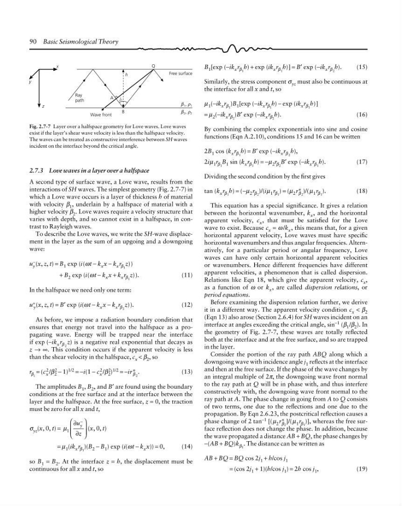
Fig. 2.7-7 Layer over a halfspace geometry for Love waves. Love waves
exist if the layer’s shear wave velocity is less than the halfspace velocity.
The waves can be treated as constructive interference between SH waves
incident on the interface beyond the critical angle.
2.7.3 Love waves in a layer over a halfspace
A second type of surface wave, a Love wave, results from the
interactions of SH waves. The simplest geometry (Fig. 2.7-7) in
which a Love wave occurs is a layer of thickness h of material
with velocity β 1 , underlain by a halfspace of material with a
higher velocity β 2 . Love waves require a velocity structure that
varies with depth, and so cannot exist in a halfspace, in contrast to Rayleigh waves.
To describe the Love waves, we write the SH-wave displacement in the layer as the sum of an upgoing and a downgoing
wave:
u −
y (x, z, t) = B 1 exp (i(ωt − k x x − k x r β 1 z))
+ B 2 exp (i(ωt − k x x + k x r β 1 z)).
(11)
In the halfspace we need only one term:
u +
y (x, z, t) = B′ exp (i(ωt − k x x − k x r β 2 z)).
(12)
As before, we impose a radiation boundary condition that
ensures that energy not travel into the halfspace as a propagating wave. Energy will be trapped near the interface
if exp (−ik x r β 2 z) is a negative real exponential that decays as
z → ∞. This condition occurs if the apparent velocity is less
than the shear velocity in the halfspace, c x < β 2 , so
r β 2 = (c 2
x /β 2
2 − 1) 1/2 = −i(1 − c 2
x /β 2
2 ) 1/2 = −ir* β 2 .
(13)
The amplitudes B 1 , B 2 , and B′ are found using the boundary
conditions at the free surface and at the interface between the
layer and the halfspace. At the free surface, z = 0, the traction
must be zero for all x and t,
σ yz (x, 0, t) = µ 1
∂
∂
u
z
y
−
⎛
⎝
⎜
⎜
⎞
⎠
⎟
⎟
(x, 0, t)
= µ 1 (ik x r β 1 )(B 2 − B 1 ) exp (i(ωt − k x x)) = 0,
(14)
so B 1 = B 2 . At the interface z = h, the displacement must be
continuous for all x and t, so
B 1 [exp (−ik x r β 1 h) + exp (ik x r β 1 h)] = B′ exp (−ik x r β 2 h).
(15)
Similarly, the stress component σ yz must also be continuous at
the interface for all x and t, so
µ 1 (−ik x r β 1 )B 1 [exp (−ik x r β 1 h) − exp (ik x r β 1 h)]
= µ 2 (−ik x r β 2 )B′ exp (−ik x r β 2 h).
(16)
By combining the complex exponentials into sine and cosine
functions (Eqn A.2.10), conditions 15 and 16 can be written
2B 1 cos (k x r β 1 h) = B′ exp (−ik x r β 2 h),
2iµ 1 r β 1 B 1 sin (k x r β 1 h) = −µ 2 r β 2 B′ exp (−ik x r β 1 h).
(17)
Dividing the second condition by the first gives
tan (k x r β 1 h) = (−µ 2 r β 2 )/(iµ 1 r β 1 ) = (µ 2 r* β 2 )/(µ 1 r β 1 ).
(18)
This equation has a special significance. It gives a relation
between the horizontal wavenumber, k x , and the horizontal
apparent velocity, c x , that must be satisfied for the Love
wave to exist. Because c x = ω /k x , this means that, for a given
horizontal apparent velocity, Love waves must have specific
horizontal wavenumbers and thus angular frequencies. Alternatively, for a particular period or angular frequency, Love
waves can have only certain horizontal apparent velocities
or wavenumbers. Hence different frequencies have different
apparent velocities, a phenomenon that is called dispersion.
Relations like Eqn 18, which give the apparent velocity, c x ,
as a function of ω or k x , are called dispersion relations, or
period equations.
Before examining the dispersion relation further, we derive
it in a different way. The apparent velocity condition c x < β 2
(Eqn 13) also arose (Section 2.6.4) for SH waves incident on an
interface at angles exceeding the critical angle, sin −1 (β 1 /β 2 ). In
the geometry of Fig. 2.7-7, these waves are totally reflected
both at the interface and at the free surface, and so are trapped
in the layer.
Consider the portion of the ray path ABQ along which a
downgoing wave with incidence angle j 1 reflects at the interface
and then at the free surface. If the phase of the wave changes by
an integral multiple of 2π, the downgoing wave front normal
to the ray path at Q will be in phase with, and thus interfere
constructively with, the downgoing wave front normal to the
ray path at A. The phase change in going from A to Q consists
of two terms, one due to the reflections and one due to the
propagation. By Eqn 2.6.23, the postcritical reflection causes a
phase change of 2 tan −1 [(µ 2 r* β 2 ]/(µ 1 r β 1 )], whereas the free surface reflection does not change the phase. In addition, because
the wave propagated a distance AB + BQ, the phase changes by
−(AB + BQ)k β 1 . The distance can be written as
AB + BQ = BQ cos 2j 1 + h/cos j 1
= (cos 2j 1 + 1)(h/cos j 1 ) = 2h cos j 1 ,
(19)
2 , 2
β
Free surface
ρ
1 , 1
β ρ
j 1
A
h
x
y
z
Ray
path
Wave front
Q
B
Fig. 2.7-7 Layer over a halfspace geometry for Love waves. Love waves
exist if the layer’s shear wave velocity is less than the halfspace velocity.
The waves can be treated as constructive interference between SH waves
incident on the interface beyond the critical angle.
2.7.3 Love waves in a layer over a halfspace
A second type of surface wave, a Love wave, results from the
interactions of SH waves. The simplest geometry (Fig. 2.7-7) in
which a Love wave occurs is a layer of thickness h of material
with velocity β 1 , underlain by a halfspace of material with a
higher velocity β 2 . Love waves require a velocity structure that
varies with depth, and so cannot exist in a halfspace, in contrast to Rayleigh waves.
To describe the Love waves, we write the SH-wave displacement in the layer as the sum of an upgoing and a downgoing
wave:
u −
y (x, z, t) = B 1 exp (i(ωt − k x x − k x r β 1 z))
+ B 2 exp (i(ωt − k x x + k x r β 1 z)).
(11)
In the halfspace we need only one term:
u +
y (x, z, t) = B′ exp (i(ωt − k x x − k x r β 2 z)).
(12)
As before, we impose a radiation boundary condition that
ensures that energy not travel into the halfspace as a propagating wave. Energy will be trapped near the interface
if exp (−ik x r β 2 z) is a negative real exponential that decays as
z → ∞. This condition occurs if the apparent velocity is less
than the shear velocity in the halfspace, c x < β 2 , so
r β 2 = (c 2
x /β 2
2 − 1) 1/2 = −i(1 − c 2
x /β 2
2 ) 1/2 = −ir* β 2 .
(13)
The amplitudes B 1 , B 2 , and B′ are found using the boundary
conditions at the free surface and at the interface between the
layer and the halfspace. At the free surface, z = 0, the traction
must be zero for all x and t,
σ yz (x, 0, t) = µ 1
∂
∂
u
z
y
−
⎛
⎝
⎜
⎜
⎞
⎠
⎟
⎟
(x, 0, t)
= µ 1 (ik x r β 1 )(B 2 − B 1 ) exp (i(ωt − k x x)) = 0,
(14)
so B 1 = B 2 . At the interface z = h, the displacement must be
continuous for all x and t, so