

84
M. D. Alba-Rodríguez et al.
Table 7 Efficiency factors in
the application of irrigation
water [16]
Efficiency app. type of irrigation (Ea) Minimum Maximum
Irrigation located underground
0.95
0.95
Irrigation located on the surface
0.90
0.90
Diffusers and micro-sprinklers
0.80
0.80
Sprinklers
0.70
0.80
Surface
0.50
0.65
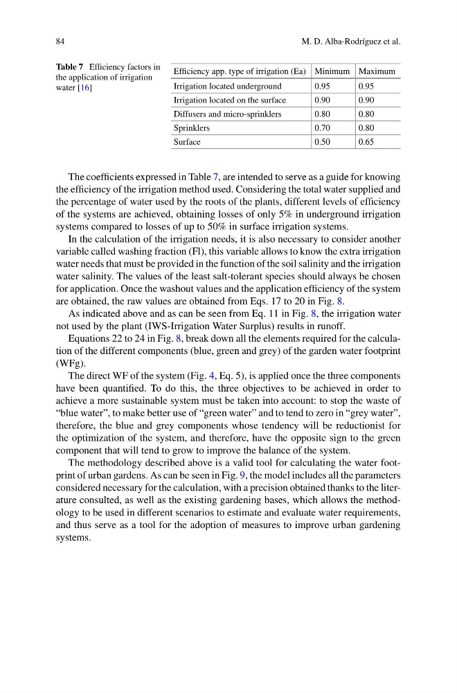
The coefficients expressed in Table 7, are intended to serve as a guide for knowing
the efficiency of the irrigation method used. Considering the total water supplied and
the percentage of water used by the roots of the plants, different levels of efficiency
of the systems are achieved, obtaining losses of only 5% in underground irrigation
systems compared to losses of up to 50% in surface irrigation systems.
In the calculation of the irrigation needs, it is also necessary to consider another
variable called washing fraction (Fl), this variable allows to know the extra irrigation
water needs that must be provided in the function of the soil salinity and the irrigation
water salinity. The values of the least salt-tolerant species should always be chosen
for application. Once the washout values and the application efficiency of the system
are obtained, the raw values are obtained from Eqs. 17 to 20 in Fig. 8.
As indicated above and as can be seen from Eq. 11 in Fig. 8, the irrigation water
not used by the plant (IWS-Irrigation Water Surplus) results in runoff.
Equations 22 to 24 in Fig. 8, break down all the elements required for the calculation of the different components (blue, green and grey) of the garden water footprint
(WFg).
The direct WF of the system (Fig. 4, Eq. 5), is applied once the three components
have been quantified. To do this, the three objectives to be achieved in order to
achieve a more sustainable system must be taken into account: to stop the waste of
“blue water”, to make better use of “green water” and to tend to zero in “grey water”,
therefore, the blue and grey components whose tendency will be reductionist for
the optimization of the system, and therefore, have the opposite sign to the green
component that will tend to grow to improve the balance of the system.
The methodology described above is a valid tool for calculating the water footprint of urban gardens. As can be seen in Fig. 9, the model includes all the parameters
considered necessary for the calculation, with a precision obtained thanks to the literature consulted, as well as the existing gardening bases, which allows the methodology to be used in different scenarios to estimate and evaluate water requirements,
and thus serve as a tool for the adoption of measures to improve urban gardening
systems.
M. D. Alba-Rodríguez et al.
Table 7 Efficiency factors in
the application of irrigation
water [16]
Efficiency app. type of irrigation (Ea) Minimum Maximum
Irrigation located underground
0.95
0.95
Irrigation located on the surface
0.90
0.90
Diffusers and micro-sprinklers
0.80
0.80
Sprinklers
0.70
0.80
Surface
0.50
0.65
The coefficients expressed in Table 7, are intended to serve as a guide for knowing
the efficiency of the irrigation method used. Considering the total water supplied and
the percentage of water used by the roots of the plants, different levels of efficiency
of the systems are achieved, obtaining losses of only 5% in underground irrigation
systems compared to losses of up to 50% in surface irrigation systems.
In the calculation of the irrigation needs, it is also necessary to consider another
variable called washing fraction (Fl), this variable allows to know the extra irrigation
water needs that must be provided in the function of the soil salinity and the irrigation
water salinity. The values of the least salt-tolerant species should always be chosen
for application. Once the washout values and the application efficiency of the system
are obtained, the raw values are obtained from Eqs. 17 to 20 in Fig. 8.
As indicated above and as can be seen from Eq. 11 in Fig. 8, the irrigation water
not used by the plant (IWS-Irrigation Water Surplus) results in runoff.
Equations 22 to 24 in Fig. 8, break down all the elements required for the calculation of the different components (blue, green and grey) of the garden water footprint
(WFg).
The direct WF of the system (Fig. 4, Eq. 5), is applied once the three components
have been quantified. To do this, the three objectives to be achieved in order to
achieve a more sustainable system must be taken into account: to stop the waste of
“blue water”, to make better use of “green water” and to tend to zero in “grey water”,
therefore, the blue and grey components whose tendency will be reductionist for
the optimization of the system, and therefore, have the opposite sign to the green
component that will tend to grow to improve the balance of the system.
The methodology described above is a valid tool for calculating the water footprint of urban gardens. As can be seen in Fig. 9, the model includes all the parameters
considered necessary for the calculation, with a precision obtained thanks to the literature consulted, as well as the existing gardening bases, which allows the methodology to be used in different scenarios to estimate and evaluate water requirements,
and thus serve as a tool for the adoption of measures to improve urban gardening
systems.