

156
7 Liquid Crystals
c
r
r
Fig. 7.6 Image of the geometrical change (from spindle to anti-spindle via cylinder) for a non-polar
molecule having the axial symmetry. r c (=
9
79 for the potential expressed by Eq. 7.17) is a threshold
for twist. Reproduced from J. Phys. Soc. Jpn., 86, 084602 (2017) [19]
1.5
1.0
0.5
0.0
T
/ V0
1.0
0.5
0.0
r
disordered
uniaxial
(nematic)
alternate
SB 1
SB 2
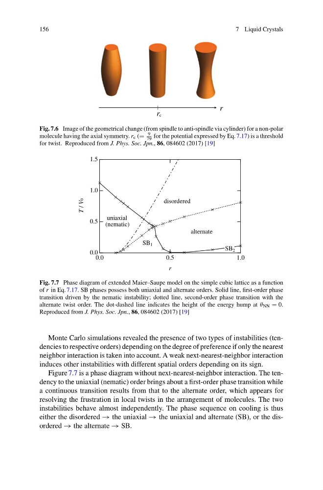
Fig. 7.7 Phase diagram of extended Maier–Saupe model on the simple cubic lattice as a function
of r in Eq. 7.17. SB phases possess both uniaxial and alternate orders. Solid line, first-order phase
transition driven by the nematic instability; dotted line, second-order phase transition with the
alternate twist order. The dot-dashed line indicates the height of the energy hump at θ NN = 0.
Reproduced from J. Phys. Soc. Jpn., 86, 084602 (2017) [19]
Monte Carlo simulations revealed the presence of two types of instabilities (tendencies to respective orders) depending on the degree of preference if only the nearest
neighbor interaction is taken into account. A weak next-nearest-neighbor interaction
induces other instabilities with different spatial orders depending on its sign.
Figure 7.7 is a phase diagram without next-nearest-neighbor interaction. The tendency to the uniaxial (nematic) order brings about a first-order phase transition while
a continuous transition results from that to the alternate order, which appears for
resolving the frustration in local twists in the arrangement of molecules. The two
instabilities behave almost independently. The phase sequence on cooling is thus
either the disordered → the uniaxial → the uniaxial and alternate (SB), or the disordered → the alternate → SB.
7 Liquid Crystals
c
r
r
Fig. 7.6 Image of the geometrical change (from spindle to anti-spindle via cylinder) for a non-polar
molecule having the axial symmetry. r c (=
9
79 for the potential expressed by Eq. 7.17) is a threshold
for twist. Reproduced from J. Phys. Soc. Jpn., 86, 084602 (2017) [19]
1.5
1.0
0.5
0.0
T
/ V0
1.0
0.5
0.0
r
disordered
uniaxial
(nematic)
alternate
SB 1
SB 2
Fig. 7.7 Phase diagram of extended Maier–Saupe model on the simple cubic lattice as a function
of r in Eq. 7.17. SB phases possess both uniaxial and alternate orders. Solid line, first-order phase
transition driven by the nematic instability; dotted line, second-order phase transition with the
alternate twist order. The dot-dashed line indicates the height of the energy hump at θ NN = 0.
Reproduced from J. Phys. Soc. Jpn., 86, 084602 (2017) [19]
Monte Carlo simulations revealed the presence of two types of instabilities (tendencies to respective orders) depending on the degree of preference if only the nearest
neighbor interaction is taken into account. A weak next-nearest-neighbor interaction
induces other instabilities with different spatial orders depending on its sign.
Figure 7.7 is a phase diagram without next-nearest-neighbor interaction. The tendency to the uniaxial (nematic) order brings about a first-order phase transition while
a continuous transition results from that to the alternate order, which appears for
resolving the frustration in local twists in the arrangement of molecules. The two
instabilities behave almost independently. The phase sequence on cooling is thus
either the disordered → the uniaxial → the uniaxial and alternate (SB), or the disordered → the alternate → SB.