

126
S. Roy and A. Chatterjee
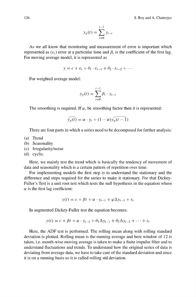
y p (t) =
i−1
i=0
y t−i
As we all know that monitoring and measurement of error is important which
represented as (ε t ) error at a particular time and β i is the coefficient of the first lag.
For moving average model, it is represented as
y = c + ε t + θ 1 · ε t−1 + θ 2 · ε t−2 + · · ·
For weighted average model:
y p (t) =
i−1
i=0
β i · y t−i
The smoothing is required. If α, be smoothing factor then it is represented:
y p (t)
= α · y t + (1 − α)y p (t − 1)
There are four parts in which a series need to be decomposed for further analysis:
(a) Trend
(b) Seasonality
(c) Irregularity/noise
(d) cyclic.
Here, we mainly test the trend which is basically the tendency of movement of
data and seasonality which is a certain pattern of repetition over time.
For implementing models the first step is to understand the stationary and the
difference and steps required for the series to make it stationary. For that DickeyFuller’s Test is a unit root test which tests the null hypothesis in the equation where
α is the first lag coefficient:
y(t) = c + βt + α · y t−1 + ϕϕy t−1 + ε t
In augmented Dickey-Fuller test the equation becomes:
y(t) = c + βt + α · y t−1 + θ 1 y t−1 + θ 2 y t−2 + · · · + ε t
Here, the ADF test is performed. The rolling mean along with rolling standard
deviation is plotted. Rolling mean is the running average and here window of 12 is
taken, i.e. month-wise moving average is taken to make a finite impulse filter and to
understand fluctuations and trends. To understand how the original series of data is
deviating from average data, we have to take care of the standard deviation and since
it is on a running basis so it is called rolling std deviation.
S. Roy and A. Chatterjee
y p (t) =
i−1
i=0
y t−i
As we all know that monitoring and measurement of error is important which
represented as (ε t ) error at a particular time and β i is the coefficient of the first lag.
For moving average model, it is represented as
y = c + ε t + θ 1 · ε t−1 + θ 2 · ε t−2 + · · ·
For weighted average model:
y p (t) =
i−1
i=0
β i · y t−i
The smoothing is required. If α, be smoothing factor then it is represented:
y p (t)
= α · y t + (1 − α)y p (t − 1)
There are four parts in which a series need to be decomposed for further analysis:
(a) Trend
(b) Seasonality
(c) Irregularity/noise
(d) cyclic.
Here, we mainly test the trend which is basically the tendency of movement of
data and seasonality which is a certain pattern of repetition over time.
For implementing models the first step is to understand the stationary and the
difference and steps required for the series to make it stationary. For that DickeyFuller’s Test is a unit root test which tests the null hypothesis in the equation where
α is the first lag coefficient:
y(t) = c + βt + α · y t−1 + ϕϕy t−1 + ε t
In augmented Dickey-Fuller test the equation becomes:
y(t) = c + βt + α · y t−1 + θ 1 y t−1 + θ 2 y t−2 + · · · + ε t
Here, the ADF test is performed. The rolling mean along with rolling standard
deviation is plotted. Rolling mean is the running average and here window of 12 is
taken, i.e. month-wise moving average is taken to make a finite impulse filter and to
understand fluctuations and trends. To understand how the original series of data is
deviating from average data, we have to take care of the standard deviation and since
it is on a running basis so it is called rolling std deviation.