

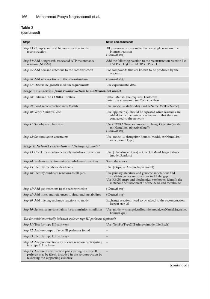
Table 2
(continued)
Steps
Notes and commands
Step 33: Compile and add biomass reaction to the
reconstruction
All precursors are assembled in one single reaction: the
biomass reaction
(Critical step)
Step 34: Add nongrowth-associated ATP maintenance
reaction (NGAM)
Add the following reaction to the reconstruction reaction list:
1ATP + 1H 2 O ! 1ADP + 1Pi + 1H
+
Step 35: Add demand reactions to the reconstruction
For compounds that are known to be produced by the
organism
Step 36: Add sink reactions to the reconstruction
(Critical step)
Step 37: Determine growth medium requirements
Use experimental data
Stage 3: Conversion from reconstruction to mathematical model
Step 38: Initialize the COBRA Toolbox
Install Matlab, the required Toolboxes
Enter this command: initCobraToolbox
Step 39: Load reconstruction into Matlab
Use: model ¼ xls2model(RxnFileName,MetFileName)
Step 40: Verify S matrix. Use
Use: spy(matrix). should be repeated when reactions are
added to the reconstruction to ensure that they are
connected to the network
Step 41: Set objective function
Use COBRA Toolbox: model ¼ changeObjective(model,
rxnNameList, objectiveCoeff)
(Critical step)
Step 42: Set simulation constraints
Use: model ¼ changeRxnBounds(model, rxnNameList,
value,boundType)
Stage 4: Network evaluation ¼ “Debugging mode”
Step 43: Check for stoichiometrically unbalanced reactions
Use: [UnbalancedRxns] ¼ CheckmMassChargeBalance
(model,RxnList)
Step 44: Evaluate stoichiometrically unbalanced reactions
Solve the errors
Step 45: Identify metabolic dead ends
Use: [Gaps] ¼ AnalyzeGaps(model)
Step 46: Identify candidate reactions to fill gaps
Use primary literature and genome annotation: find
candidate genes and reactions to fill the gap
Use KEGG maps and biochemical textbooks: identify the
metabolic “environment” of the dead-end metabolite
Step 47: Add gap reactions to the reconstruction
(Critical step)
Step 48: Add notes and references to dead-end metabolites
(Critical step)
Step 49: Add missing exchange reactions to model
Exchange reactions need to be added to the reconstruction.
Repeat step 21
Step 50: Set exchange constraints for a simulation condition Use: model ¼ changeRxnBounds(model,rxnNameList,value,
boundType)
Test for stoichiometrically balanced cycles or type III pathways (optional)
Step 51: Test for type III pathways
Use: TestForTypeIIIPathways(model,ListExch)
Step 52: Analyze output if type III pathways found
–
Step 53: Identify type III pathways
–
Step 54: Analyze directionality of each reaction participating
in a type III pathway
–
Step 55: Analyze if any reaction participating in a type III
pathway may be falsely included in the reconstruction by
reviewing the supporting evidence
–
(continued)
166
Mohammad Pooya Naghshbandi et al.
(continued)
Steps
Notes and commands
Step 33: Compile and add biomass reaction to the
reconstruction
All precursors are assembled in one single reaction: the
biomass reaction
(Critical step)
Step 34: Add nongrowth-associated ATP maintenance
reaction (NGAM)
Add the following reaction to the reconstruction reaction list:
1ATP + 1H 2 O ! 1ADP + 1Pi + 1H
+
Step 35: Add demand reactions to the reconstruction
For compounds that are known to be produced by the
organism
Step 36: Add sink reactions to the reconstruction
(Critical step)
Step 37: Determine growth medium requirements
Use experimental data
Stage 3: Conversion from reconstruction to mathematical model
Step 38: Initialize the COBRA Toolbox
Install Matlab, the required Toolboxes
Enter this command: initCobraToolbox
Step 39: Load reconstruction into Matlab
Use: model ¼ xls2model(RxnFileName,MetFileName)
Step 40: Verify S matrix. Use
Use: spy(matrix). should be repeated when reactions are
added to the reconstruction to ensure that they are
connected to the network
Step 41: Set objective function
Use COBRA Toolbox: model ¼ changeObjective(model,
rxnNameList, objectiveCoeff)
(Critical step)
Step 42: Set simulation constraints
Use: model ¼ changeRxnBounds(model, rxnNameList,
value,boundType)
Stage 4: Network evaluation ¼ “Debugging mode”
Step 43: Check for stoichiometrically unbalanced reactions
Use: [UnbalancedRxns] ¼ CheckmMassChargeBalance
(model,RxnList)
Step 44: Evaluate stoichiometrically unbalanced reactions
Solve the errors
Step 45: Identify metabolic dead ends
Use: [Gaps] ¼ AnalyzeGaps(model)
Step 46: Identify candidate reactions to fill gaps
Use primary literature and genome annotation: find
candidate genes and reactions to fill the gap
Use KEGG maps and biochemical textbooks: identify the
metabolic “environment” of the dead-end metabolite
Step 47: Add gap reactions to the reconstruction
(Critical step)
Step 48: Add notes and references to dead-end metabolites
(Critical step)
Step 49: Add missing exchange reactions to model
Exchange reactions need to be added to the reconstruction.
Repeat step 21
Step 50: Set exchange constraints for a simulation condition Use: model ¼ changeRxnBounds(model,rxnNameList,value,
boundType)
Test for stoichiometrically balanced cycles or type III pathways (optional)
Step 51: Test for type III pathways
Use: TestForTypeIIIPathways(model,ListExch)
Step 52: Analyze output if type III pathways found
–
Step 53: Identify type III pathways
–
Step 54: Analyze directionality of each reaction participating
in a type III pathway
–
Step 55: Analyze if any reaction participating in a type III
pathway may be falsely included in the reconstruction by
reviewing the supporting evidence
–
(continued)
166
Mohammad Pooya Naghshbandi et al.