

66
4 Testing and Validating Against Historic Spills
A brief description and examples of each type of dataset is given below.
Surface resource datasets
Three methods were used to estimate VEC densities and construct resource data sets
used in the ERA Acute modelling. The two first methods were used for the DHOS
incident and the third for the EVOS incident. Different methods are used based on
different availability of suitable datasets.
The first method used estimates of VEC densities in the study area (Deepwater
Horizon Natural Resource Damage Assessment Trustees 2016; Haney et al. 2014a,
b) combined with probability distributions and Monte Carlo Simulations. Different
densities and probability distributions were used for distinct habitat types within
the study area. Each density and habitat were assigned a log-normal distribution
with a standard deviation equal to 1.5 times the density (mean). The distribution
of organisms in the environment is often log-normal and in most plant and animal
communities, the abundance of species follows a (truncated) log-normal distribution
(e.g. Limpert et al. 2001). A random number was drawn from the probability distribution, representing the abundance of the VEC in that cell. The same process was
repeated until all grid cells in the study area were filled, and then repeated 500 times
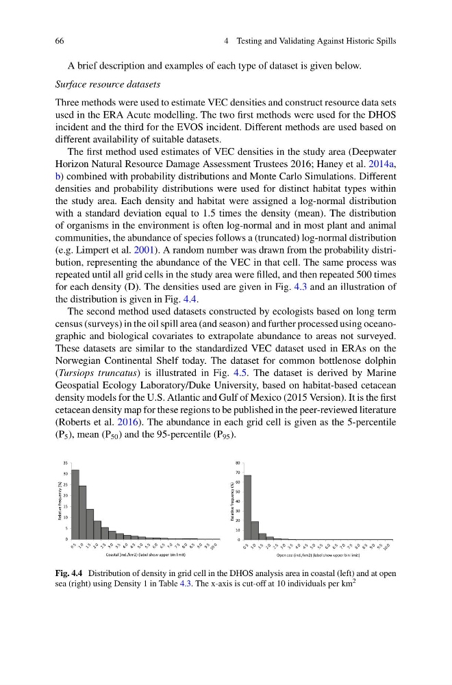
for each density (D). The densities used are given in Fig. 4.3 and an illustration of
the distribution is given in Fig. 4.4.
The second method used datasets constructed by ecologists based on long term
census (surveys) in the oil spill area (and season) and further processed using oceanographic and biological covariates to extrapolate abundance to areas not surveyed.
These datasets are similar to the standardized VEC dataset used in ERAs on the
Norwegian Continental Shelf today. The dataset for common bottlenose dolphin
(Tursiops truncatus) is illustrated in Fig. 4.5. The dataset is derived by Marine
Geospatial Ecology Laboratory/Duke University, based on habitat-based cetacean
density models for the U.S. Atlantic and Gulf of Mexico (2015 Version). It is the first
cetacean density map for these regions to be published in the peer-reviewed literature
(Roberts et al. 2016). The abundance in each grid cell is given as the 5-percentile
(P 5 ), mean (P 50 ) and the 95-percentile (P 95 ).
0
5
10
15
20
25
30
35
Relative frequency (%)
Coastal (ind./km2) (label show upper bin limit)
0
10
20
30
40
50
60
70
80
Relative frequency (%)
Open sea (ind./km2) (label show upper bin limit)
Fig. 4.4 Distribution of density in grid cell in the DHOS analysis area in coastal (left) and at open
sea (right) using Density 1 in Table 4.3. The x-axis is cut-off at 10 individuals per km 2
4 Testing and Validating Against Historic Spills
A brief description and examples of each type of dataset is given below.
Surface resource datasets
Three methods were used to estimate VEC densities and construct resource data sets
used in the ERA Acute modelling. The two first methods were used for the DHOS
incident and the third for the EVOS incident. Different methods are used based on
different availability of suitable datasets.
The first method used estimates of VEC densities in the study area (Deepwater
Horizon Natural Resource Damage Assessment Trustees 2016; Haney et al. 2014a,
b) combined with probability distributions and Monte Carlo Simulations. Different
densities and probability distributions were used for distinct habitat types within
the study area. Each density and habitat were assigned a log-normal distribution
with a standard deviation equal to 1.5 times the density (mean). The distribution
of organisms in the environment is often log-normal and in most plant and animal
communities, the abundance of species follows a (truncated) log-normal distribution
(e.g. Limpert et al. 2001). A random number was drawn from the probability distribution, representing the abundance of the VEC in that cell. The same process was
repeated until all grid cells in the study area were filled, and then repeated 500 times
for each density (D). The densities used are given in Fig. 4.3 and an illustration of
the distribution is given in Fig. 4.4.
The second method used datasets constructed by ecologists based on long term
census (surveys) in the oil spill area (and season) and further processed using oceanographic and biological covariates to extrapolate abundance to areas not surveyed.
These datasets are similar to the standardized VEC dataset used in ERAs on the
Norwegian Continental Shelf today. The dataset for common bottlenose dolphin
(Tursiops truncatus) is illustrated in Fig. 4.5. The dataset is derived by Marine
Geospatial Ecology Laboratory/Duke University, based on habitat-based cetacean
density models for the U.S. Atlantic and Gulf of Mexico (2015 Version). It is the first
cetacean density map for these regions to be published in the peer-reviewed literature
(Roberts et al. 2016). The abundance in each grid cell is given as the 5-percentile
(P 5 ), mean (P 50 ) and the 95-percentile (P 95 ).
0
5
10
15
20
25
30
35
Relative frequency (%)
Coastal (ind./km2) (label show upper bin limit)
0
10
20
30
40
50
60
70
80
Relative frequency (%)
Open sea (ind./km2) (label show upper bin limit)
Fig. 4.4 Distribution of density in grid cell in the DHOS analysis area in coastal (left) and at open
sea (right) using Density 1 in Table 4.3. The x-axis is cut-off at 10 individuals per km 2