

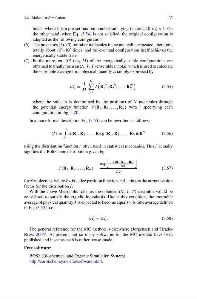
3.4 Molecular Simulations
137
holds, where ξ is a pre-set random number satisfying the range 0 < ξ < 1. On
the other hand, when Eq. (3.54) is not satisfied, the original configuration is
adopted as the following configuration.
(6) The processes (3)–(5) for other molecules in the unit cell is repeated, therefore,
totally about 10
5 –10
6 times, and the eventual configuration itself achieves the
energetically stable state.
(7) Furthermore, ca. 10
6 (say M) of the energetically stable configurations are
obtained to finally form an (N, V, T ) ensemble in total, which is used to calculate
the ensemble average for a physical quantity A simply expressed by
A =
1
M
M
j=1
A
R
(j)
1 , R
(j)
2 , . . . , R
(j)
N
(3.55)
where the value A is determined by the positions of N molecules through
the potential energy function V (R 1 , R 2 , . . . , R N ) with j specifying each
configuration in Fig. 3.20.
In a more formal description Eq. (3.55) can be rewritten as follows:
A =
A(R 1 , R 2 , . . . , R N )f (R 1 , R 2 , . . . , R N )dR
N
(3.56)
using the distribution function f often used in statistical mechanics. This f actually
signifies the Boltzmann distribution given by
f (R 1 , R 2 , . . . , R N ) =
exp
−
V (R1,R2,...,RN )
k B T
Z N
(3.57)
for N molecules, where Z N is called partition function and acting as the normalization
factor for the distribution f .
With the above Metropolis scheme, the obtained (N, V, T ) ensemble would be
considered to satisfy the ergodic hypothesis. Under this condition, the ensemble
average of physical quantity A is expected to become equal to its time average defined
in Eq. (3.53), i.e.,
A = A t
(3.58)
The general reference for the MC method is elsewhere (Jorgensen and TiradoRives 2005). At present, not so many softwares for the MC method have been
published and it seems each is rather house-made.
Free software:
BOSS (Biochemical and Organic Simulation System).
http://zarbi.chem.yale.edu/software.html.
137
holds, where ξ is a pre-set random number satisfying the range 0 < ξ < 1. On
the other hand, when Eq. (3.54) is not satisfied, the original configuration is
adopted as the following configuration.
(6) The processes (3)–(5) for other molecules in the unit cell is repeated, therefore,
totally about 10
5 –10
6 times, and the eventual configuration itself achieves the
energetically stable state.
(7) Furthermore, ca. 10
6 (say M) of the energetically stable configurations are
obtained to finally form an (N, V, T ) ensemble in total, which is used to calculate
the ensemble average for a physical quantity A simply expressed by
A =
1
M
M
j=1
A
R
(j)
1 , R
(j)
2 , . . . , R
(j)
N
(3.55)
where the value A is determined by the positions of N molecules through
the potential energy function V (R 1 , R 2 , . . . , R N ) with j specifying each
configuration in Fig. 3.20.
In a more formal description Eq. (3.55) can be rewritten as follows:
A =
A(R 1 , R 2 , . . . , R N )f (R 1 , R 2 , . . . , R N )dR
N
(3.56)
using the distribution function f often used in statistical mechanics. This f actually
signifies the Boltzmann distribution given by
f (R 1 , R 2 , . . . , R N ) =
exp
−
V (R1,R2,...,RN )
k B T
Z N
(3.57)
for N molecules, where Z N is called partition function and acting as the normalization
factor for the distribution f .
With the above Metropolis scheme, the obtained (N, V, T ) ensemble would be
considered to satisfy the ergodic hypothesis. Under this condition, the ensemble
average of physical quantity A is expected to become equal to its time average defined
in Eq. (3.53), i.e.,
A = A t
(3.58)
The general reference for the MC method is elsewhere (Jorgensen and TiradoRives 2005). At present, not so many softwares for the MC method have been
published and it seems each is rather house-made.
Free software:
BOSS (Biochemical and Organic Simulation System).
http://zarbi.chem.yale.edu/software.html.