

136
3 Fundamentals of the Analysis Tools
2α
2α
Original configuraƟon
Following configuraƟon 1
Following configuraƟon 2
Final configuraƟon
FormaƟon of ensemble
M
1
2
3
4
………………………..
………………………..
…………………
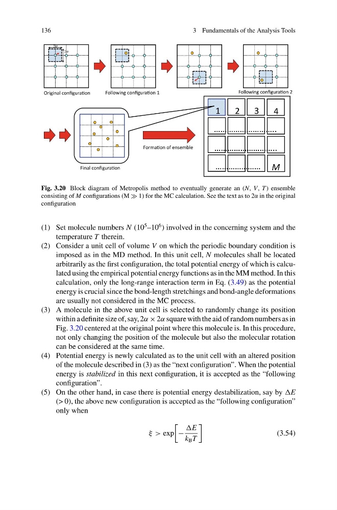
Fig. 3.20 Block diagram of Metropolis method to eventually generate an (N, V, T ) ensemble
consisting of M configurations (M 1) for the MC calculation. See the text as to 2α in the original
configuration
(1) Set molecule numbers N (10
5 –10
6 ) involved in the concerning system and the
temperature T therein.
(2) Consider a unit cell of volume V on which the periodic boundary condition is
imposed as in the MD method. In this unit cell, N molecules shall be located
arbitrarily as the first configuration, the total potential energy of which is calculated using the empirical potential energy functions as in the MM method. In this
calculation, only the long-range interaction term in Eq. (3.49) as the potential
energy is crucial since the bond-length stretchings and bond-angle deformations
are usually not considered in the MC process.
(3) A molecule in the above unit cell is selected to randomly change its position
within a definite size of, say, 2α × 2α square with the aid of random numbers as in
Fig. 3.20 centered at the original point where this molecule is. In this procedure,
not only changing the position of the molecule but also the molecular rotation
can be considered at the same time.
(4) Potential energy is newly calculated as to the unit cell with an altered position
of the molecule described in (3) as the “next configuration”. When the potential
energy is stabilized in this next configuration, it is accepted as the “following
configuration”.
(5) On the other hand, in case there is potential energy destabilization, say by
(> 0), the above new configuration is accepted as the “following configuration”
only when
ξ > exp
−
k B T
(3.54)
3 Fundamentals of the Analysis Tools
2α
2α
Original configuraƟon
Following configuraƟon 1
Following configuraƟon 2
Final configuraƟon
FormaƟon of ensemble
M
1
2
3
4
………………………..
………………………..
…………………
Fig. 3.20 Block diagram of Metropolis method to eventually generate an (N, V, T ) ensemble
consisting of M configurations (M 1) for the MC calculation. See the text as to 2α in the original
configuration
(1) Set molecule numbers N (10
5 –10
6 ) involved in the concerning system and the
temperature T therein.
(2) Consider a unit cell of volume V on which the periodic boundary condition is
imposed as in the MD method. In this unit cell, N molecules shall be located
arbitrarily as the first configuration, the total potential energy of which is calculated using the empirical potential energy functions as in the MM method. In this
calculation, only the long-range interaction term in Eq. (3.49) as the potential
energy is crucial since the bond-length stretchings and bond-angle deformations
are usually not considered in the MC process.
(3) A molecule in the above unit cell is selected to randomly change its position
within a definite size of, say, 2α × 2α square with the aid of random numbers as in
Fig. 3.20 centered at the original point where this molecule is. In this procedure,
not only changing the position of the molecule but also the molecular rotation
can be considered at the same time.
(4) Potential energy is newly calculated as to the unit cell with an altered position
of the molecule described in (3) as the “next configuration”. When the potential
energy is stabilized in this next configuration, it is accepted as the “following
configuration”.
(5) On the other hand, in case there is potential energy destabilization, say by
(> 0), the above new configuration is accepted as the “following configuration”
only when
ξ > exp
−
k B T
(3.54)