

3.4 Molecular Simulations
135
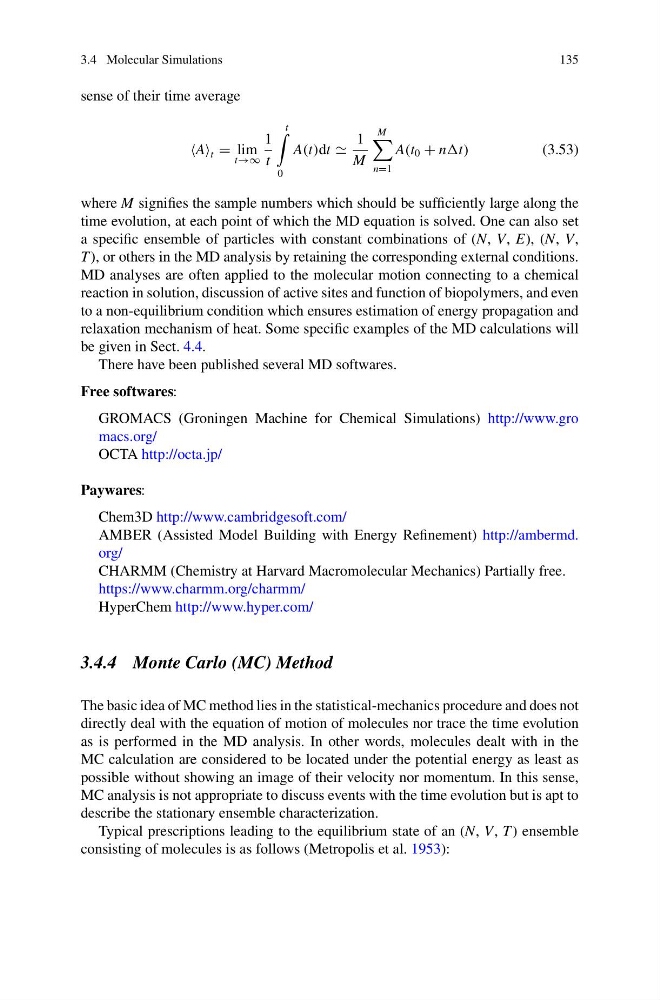
sense of their time average
A t = lim
t→∞
1
t
t
0
A(t)dt
1
M
M
n=1
A(t 0 + nt)
(3.53)
where M signifies the sample numbers which should be sufficiently large along the
time evolution, at each point of which the MD equation is solved. One can also set
a specific ensemble of particles with constant combinations of (N, V, E), (N, V,
T ), or others in the MD analysis by retaining the corresponding external conditions.
MD analyses are often applied to the molecular motion connecting to a chemical
reaction in solution, discussion of active sites and function of biopolymers, and even
to a non-equilibrium condition which ensures estimation of energy propagation and
relaxation mechanism of heat. Some specific examples of the MD calculations will
be given in Sect. 4.4.
There have been published several MD softwares.
Free softwares:
GROMACS (Groningen Machine for Chemical Simulations) http://www.gro
macs.org/
OCTA http://octa.jp/
Paywares:
Chem3D http://www.cambridgesoft.com/
AMBER (Assisted Model Building with Energy Refinement) http://ambermd.
org/
CHARMM (Chemistry at Harvard Macromolecular Mechanics) Partially free.
https://www.charmm.org/charmm/
HyperChem http://www.hyper.com/
3.4.4 Monte Carlo (MC) Method
The basic idea of MC method lies in the statistical-mechanics procedure and does not
directly deal with the equation of motion of molecules nor trace the time evolution
as is performed in the MD analysis. In other words, molecules dealt with in the
MC calculation are considered to be located under the potential energy as least as
possible without showing an image of their velocity nor momentum. In this sense,
MC analysis is not appropriate to discuss events with the time evolution but is apt to
describe the stationary ensemble characterization.
Typical prescriptions leading to the equilibrium state of an (N, V, T ) ensemble
consisting of molecules is as follows (Metropolis et al. 1953):
135
sense of their time average
A t = lim
t→∞
1
t
t
0
A(t)dt
1
M
M
n=1
A(t 0 + nt)
(3.53)
where M signifies the sample numbers which should be sufficiently large along the
time evolution, at each point of which the MD equation is solved. One can also set
a specific ensemble of particles with constant combinations of (N, V, E), (N, V,
T ), or others in the MD analysis by retaining the corresponding external conditions.
MD analyses are often applied to the molecular motion connecting to a chemical
reaction in solution, discussion of active sites and function of biopolymers, and even
to a non-equilibrium condition which ensures estimation of energy propagation and
relaxation mechanism of heat. Some specific examples of the MD calculations will
be given in Sect. 4.4.
There have been published several MD softwares.
Free softwares:
GROMACS (Groningen Machine for Chemical Simulations) http://www.gro
macs.org/
OCTA http://octa.jp/
Paywares:
Chem3D http://www.cambridgesoft.com/
AMBER (Assisted Model Building with Energy Refinement) http://ambermd.
org/
CHARMM (Chemistry at Harvard Macromolecular Mechanics) Partially free.
https://www.charmm.org/charmm/
HyperChem http://www.hyper.com/
3.4.4 Monte Carlo (MC) Method
The basic idea of MC method lies in the statistical-mechanics procedure and does not
directly deal with the equation of motion of molecules nor trace the time evolution
as is performed in the MD analysis. In other words, molecules dealt with in the
MC calculation are considered to be located under the potential energy as least as
possible without showing an image of their velocity nor momentum. In this sense,
MC analysis is not appropriate to discuss events with the time evolution but is apt to
describe the stationary ensemble characterization.
Typical prescriptions leading to the equilibrium state of an (N, V, T ) ensemble
consisting of molecules is as follows (Metropolis et al. 1953):