

134
3 Fundamentals of the Analysis Tools
L
r c
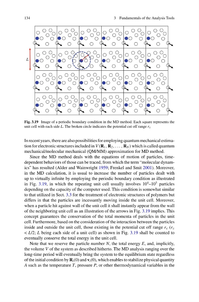
Fig. 3.19 Image of a periodic boundary condition in the MD method. Each square represents the
unit cell with each side L. The broken circle indicates the potential cut off range r c
In recent years, there are also possibilities for employing quantum mechanical estimation for electronic structures included in V (R 1 , R 2 , . . . , R N ) which is called quantum
mechanical/molecular mechanical (QM/MM) approximation for MD method.
Since the MD method deals with the equations of motion of particles, timedependent behaviors of those can be traced, from which the term “molecular dynamics” has resulted (Alder and Wainwright 1959; Frenkel and Smit 2001). Moreover,
in the MD calculation, it is usual to increase the number of particles dealt with
up to virtually infinite by employing the periodic boundary condition as illustrated
in Fig. 3.19, in which the repeating unit cell usually involves 10
4 –10
5 particles
depending on the capacity of the computer used. This condition is somewhat similar
to that utilized in Sect. 3.3 for the treatment of electronic structures of polymers but
differs in that the particles are incessantly moving inside the unit cell. Moreover,
when a particle hit against wall of the unit cell it shall instantly appear from the wall
of the neighboring unit cell as an illustration of the arrows in Fig. 3.19 implies. This
concept guarantees the conservation of the total momenta of particles in the unit
cell. Furthermore, based on the consideration of the interaction between the particles
inside and outside the unit cell, those existing in the potential cut off range r c (r c
< L/2; L being each side of a unit cell) as shown in Fig. 3.19 shall be counted to
eventually conserve the total energy in the unit cell.
Note that we reserve the particle number N, the total energy E, and, implicitly,
the volume V of the system as described hitherto. The MD analysis ranging over the
long-time period will eventually bring the system to the equilibrium state regardless
of the initial condition by R i (0) and v i (0), which enables to stabilize physical quantity
A such as the temperature T, pressure P, or other thermodynamical variables in the
3 Fundamentals of the Analysis Tools
L
r c
Fig. 3.19 Image of a periodic boundary condition in the MD method. Each square represents the
unit cell with each side L. The broken circle indicates the potential cut off range r c
In recent years, there are also possibilities for employing quantum mechanical estimation for electronic structures included in V (R 1 , R 2 , . . . , R N ) which is called quantum
mechanical/molecular mechanical (QM/MM) approximation for MD method.
Since the MD method deals with the equations of motion of particles, timedependent behaviors of those can be traced, from which the term “molecular dynamics” has resulted (Alder and Wainwright 1959; Frenkel and Smit 2001). Moreover,
in the MD calculation, it is usual to increase the number of particles dealt with
up to virtually infinite by employing the periodic boundary condition as illustrated
in Fig. 3.19, in which the repeating unit cell usually involves 10
4 –10
5 particles
depending on the capacity of the computer used. This condition is somewhat similar
to that utilized in Sect. 3.3 for the treatment of electronic structures of polymers but
differs in that the particles are incessantly moving inside the unit cell. Moreover,
when a particle hit against wall of the unit cell it shall instantly appear from the wall
of the neighboring unit cell as an illustration of the arrows in Fig. 3.19 implies. This
concept guarantees the conservation of the total momenta of particles in the unit
cell. Furthermore, based on the consideration of the interaction between the particles
inside and outside the unit cell, those existing in the potential cut off range r c (r c
< L/2; L being each side of a unit cell) as shown in Fig. 3.19 shall be counted to
eventually conserve the total energy in the unit cell.
Note that we reserve the particle number N, the total energy E, and, implicitly,
the volume V of the system as described hitherto. The MD analysis ranging over the
long-time period will eventually bring the system to the equilibrium state regardless
of the initial condition by R i (0) and v i (0), which enables to stabilize physical quantity
A such as the temperature T, pressure P, or other thermodynamical variables in the