

3.4 Molecular Simulations
133
AMBER (Assisted Model Building with Energy Refinement) http://ambermd.
org/
CHARMM (Chemistry at Harvard Macromolecular Mechanics) Partially free.
https://www.charmm.org/charmm/
CONFLEX http://www.conflex.net/
3.4.3 Molecular Dynamics (MD)
In the MD simulation of a system consisting of N particles, the equations of motion are
explicitly considered in the framework of classical mechanics described as follows:
M i
d
2 R i (t)
dt 2 = F i (t) (i = 1, 2, 3, . . . , N )
(3.50)
where M i , R i , and F i stand for, respectively, the mass, position vector, and force
applied concerning the ith particle. These equations are numerically solved based on
the difference method, in which, starting from the initial condition (information on
R i (0) and v i (0), where v i (t) stands for the velocity of the ith particle), each equation is
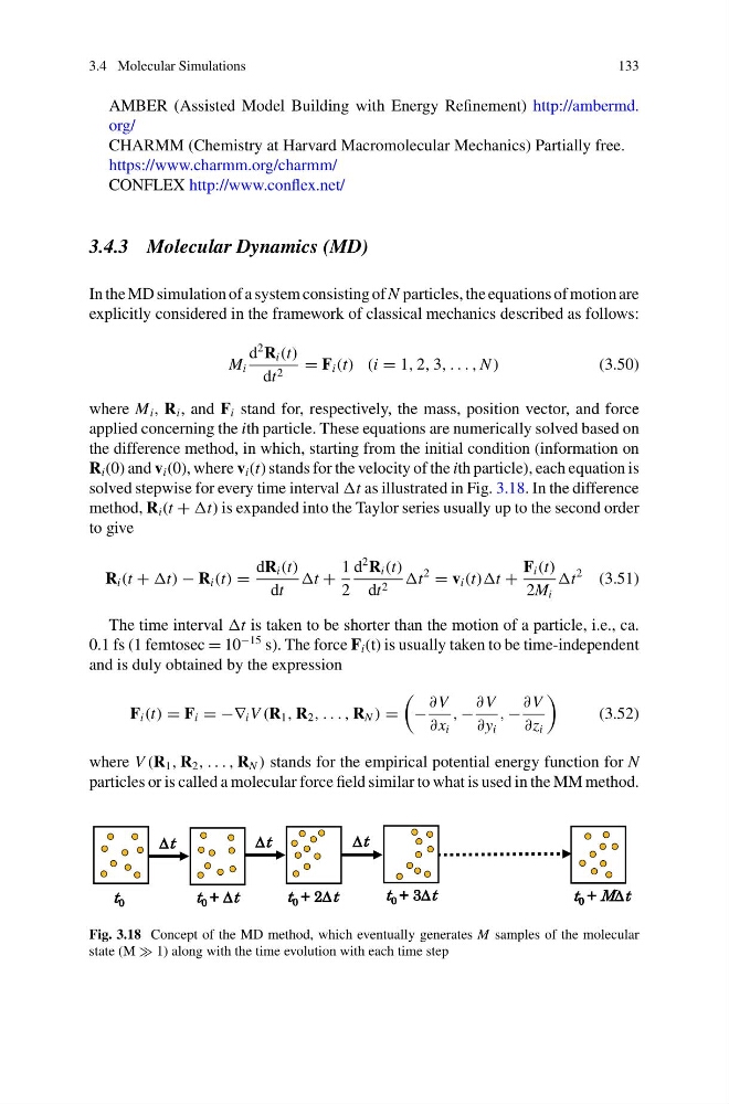
solved stepwise for every time interval as illustrated in Fig. 3.18. In the difference
method, R i (t + is expanded into the Taylor series usually up to the second order
to give
R i (t + − R i (t) =
dR i (t)
dt
+
1
2
d
2 R i (t)
dt 2
2
= v i (t))t +
F i (t)
2M i
2 (3.51)
The time interval is taken to be shorter than the motion of a particle, i.e., ca.
0.1 fs (1 femtosec = 10
−15 s). The force F i (t) is usually taken to be time-independent
and is duly obtained by the expression
F i (t) = F i = −∇ i V (R 1 , R 2 , . . . , R N ) =
−
∂ V
∂x i
, −
∂ V
∂y i
, −
∂ V
∂z i
(3.52)
where V (R 1 , R 2 , . . . , R N ) stands for the empirical potential energy function for N
particles or is called a molecular force field similar to what is used in the MM method.
t 0
Δt
t 0 + Δt
Δt
t 0 + 2Δt
Δt
t 0 + 3Δt
t 0 + MΔt
Fig. 3.18 Concept of the MD method, which eventually generates M samples of the molecular
state (M 1) along with the time evolution with each time step
133
AMBER (Assisted Model Building with Energy Refinement) http://ambermd.
org/
CHARMM (Chemistry at Harvard Macromolecular Mechanics) Partially free.
https://www.charmm.org/charmm/
CONFLEX http://www.conflex.net/
3.4.3 Molecular Dynamics (MD)
In the MD simulation of a system consisting of N particles, the equations of motion are
explicitly considered in the framework of classical mechanics described as follows:
M i
d
2 R i (t)
dt 2 = F i (t) (i = 1, 2, 3, . . . , N )
(3.50)
where M i , R i , and F i stand for, respectively, the mass, position vector, and force
applied concerning the ith particle. These equations are numerically solved based on
the difference method, in which, starting from the initial condition (information on
R i (0) and v i (0), where v i (t) stands for the velocity of the ith particle), each equation is
solved stepwise for every time interval as illustrated in Fig. 3.18. In the difference
method, R i (t + is expanded into the Taylor series usually up to the second order
to give
R i (t + − R i (t) =
dR i (t)
dt
+
1
2
d
2 R i (t)
dt 2
2
= v i (t))t +
F i (t)
2M i
2 (3.51)
The time interval is taken to be shorter than the motion of a particle, i.e., ca.
0.1 fs (1 femtosec = 10
−15 s). The force F i (t) is usually taken to be time-independent
and is duly obtained by the expression
F i (t) = F i = −∇ i V (R 1 , R 2 , . . . , R N ) =
−
∂ V
∂x i
, −
∂ V
∂y i
, −
∂ V
∂z i
(3.52)
where V (R 1 , R 2 , . . . , R N ) stands for the empirical potential energy function for N
particles or is called a molecular force field similar to what is used in the MM method.
t 0
Δt
t 0 + Δt
Δt
t 0 + 2Δt
Δt
t 0 + 3Δt
t 0 + MΔt
Fig. 3.18 Concept of the MD method, which eventually generates M samples of the molecular
state (M 1) along with the time evolution with each time step