

3.4 Molecular Simulations
131
3.4.2 Molecular Mechanics (MM)
The MM method consists of a rather simple idea in that conformation of molecules,
oligomers, or even longer polymeric chains is determined by the molecular motion
under the empirical potential energy function employed (Kollman et al. 2000).
Part of this method has already been mentioned in Sect. 2.1 used in the preliminary optimization process of molecular structure. The most important ingredient
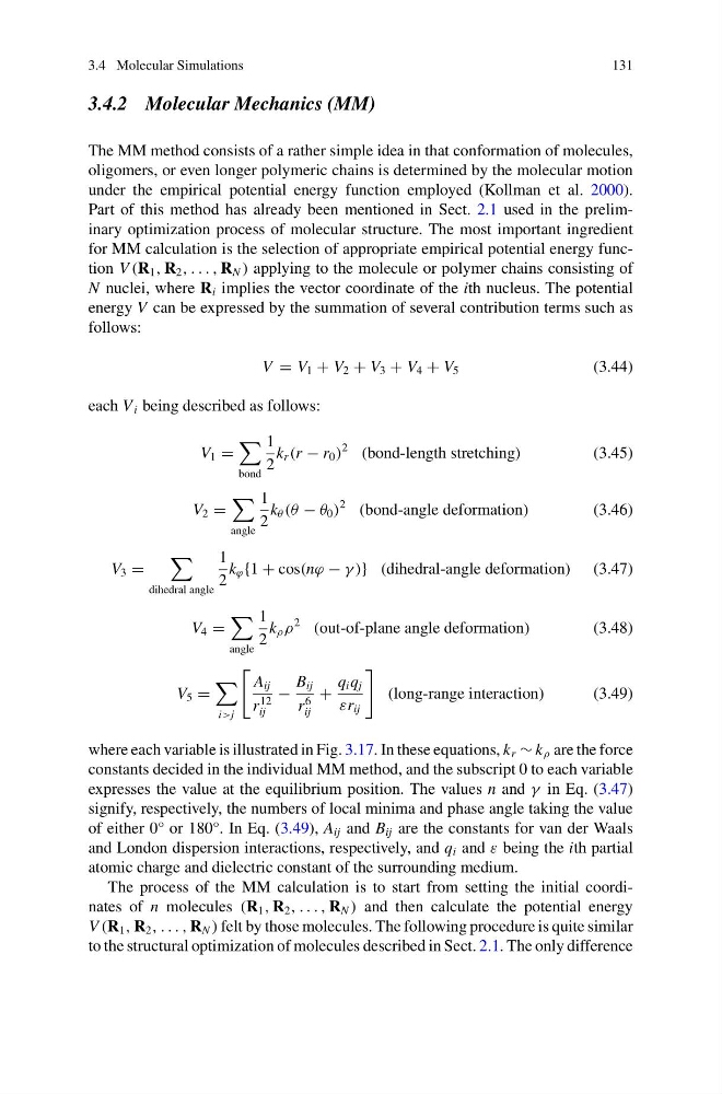
for MM calculation is the selection of appropriate empirical potential energy function V (R 1 , R 2 , . . . , R N ) applying to the molecule or polymer chains consisting of
N nuclei, where R i implies the vector coordinate of the ith nucleus. The potential
energy V can be expressed by the summation of several contribution terms such as
follows:
V = V 1 + V 2 + V 3 + V 4 + V 5
(3.44)
each V i being described as follows:
V 1 =
bond
1
2
k r (r − r 0 )
2
(bond-length stretching)
(3.45)
V 2 =
angle
1
2
k θ (θ − θ 0 )
2
(bond-angle deformation)
(3.46)
V 3 =
dihedral angle
1
2
k ϕ {1 + cos(nϕ − γ )} (dihedral-angle deformation) (3.47)
V 4 =
angle
1
2
k ρ ρ
2
(out-of-plane angle deformation)
(3.48)
V 5 =
i>j
A ij
r
12
ij
−
B ij
r
6
ij
+
q i q j
εr ij
(long-range interaction)
(3.49)
where each variable is illustrated in Fig. 3.17. In these equations, k r ∼ k ρ are the force
constants decided in the individual MM method, and the subscript 0 to each variable
expresses the value at the equilibrium position. The values n and γ in Eq. (3.47)
signify, respectively, the numbers of local minima and phase angle taking the value
of either 0° or 180°. In Eq. (3.49), A ij and B ij are the constants for van der Waals
and London dispersion interactions, respectively, and q i and ε being the ith partial
atomic charge and dielectric constant of the surrounding medium.
The process of the MM calculation is to start from setting the initial coordinates of n molecules (R 1 , R 2 , . . . , R N ) and then calculate the potential energy
V (R 1 , R 2 , . . . , R N ) felt by those molecules. The following procedure is quite similar
to the structural optimization of molecules described in Sect. 2.1. The only difference
131
3.4.2 Molecular Mechanics (MM)
The MM method consists of a rather simple idea in that conformation of molecules,
oligomers, or even longer polymeric chains is determined by the molecular motion
under the empirical potential energy function employed (Kollman et al. 2000).
Part of this method has already been mentioned in Sect. 2.1 used in the preliminary optimization process of molecular structure. The most important ingredient
for MM calculation is the selection of appropriate empirical potential energy function V (R 1 , R 2 , . . . , R N ) applying to the molecule or polymer chains consisting of
N nuclei, where R i implies the vector coordinate of the ith nucleus. The potential
energy V can be expressed by the summation of several contribution terms such as
follows:
V = V 1 + V 2 + V 3 + V 4 + V 5
(3.44)
each V i being described as follows:
V 1 =
bond
1
2
k r (r − r 0 )
2
(bond-length stretching)
(3.45)
V 2 =
angle
1
2
k θ (θ − θ 0 )
2
(bond-angle deformation)
(3.46)
V 3 =
dihedral angle
1
2
k ϕ {1 + cos(nϕ − γ )} (dihedral-angle deformation) (3.47)
V 4 =
angle
1
2
k ρ ρ
2
(out-of-plane angle deformation)
(3.48)
V 5 =
i>j
A ij
r
12
ij
−
B ij
r
6
ij
+
q i q j
εr ij
(long-range interaction)
(3.49)
where each variable is illustrated in Fig. 3.17. In these equations, k r ∼ k ρ are the force
constants decided in the individual MM method, and the subscript 0 to each variable
expresses the value at the equilibrium position. The values n and γ in Eq. (3.47)
signify, respectively, the numbers of local minima and phase angle taking the value
of either 0° or 180°. In Eq. (3.49), A ij and B ij are the constants for van der Waals
and London dispersion interactions, respectively, and q i and ε being the ith partial
atomic charge and dielectric constant of the surrounding medium.
The process of the MM calculation is to start from setting the initial coordinates of n molecules (R 1 , R 2 , . . . , R N ) and then calculate the potential energy
V (R 1 , R 2 , . . . , R N ) felt by those molecules. The following procedure is quite similar
to the structural optimization of molecules described in Sect. 2.1. The only difference