

3.2 Density Functional Theory (DFT) Calculations
113
corresponds to the first term of the Hamiltonian in Eq. (3.2) and U to the summation
of the second and the third terms. T 0 in the rightmost side of Eq. (3.20) is made
to represent the fictitious kinetic energy in the “non-interacting” electronic system
having the density (r), the third term the corresponding (classical) Coulomb energy,
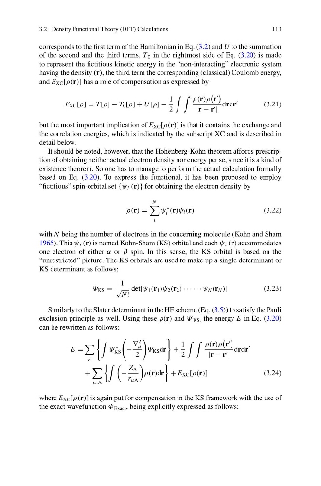
and E XC [ρ(r)] has a role of compensation as expressed by
E XC [ρ] = T [ρ] − T 0 [ρ] + U [ρ] −
1
2
ρ(r)ρ
r
|r − r |
drdr
(3.21)
but the most important implication of E XC [ρ(r)] is that it contains the exchange and
the correlation energies, which is indicated by the subscript XC and is described in
detail below.
It should be noted, however, that the Hohenberg-Kohn theorem affords prescription of obtaining neither actual electron density nor energy per se, since it is a kind of
existence theorem. So one has to manage to perform the actual calculation formally
based on Eq. (3.20). To express the functional, it has been proposed to employ
“fictitious” spin-orbital set {ψ i (r)} for obtaining the electron density by
ρ(r) =
N
i
ψ
∗
i (r)ψ i (r)
(3.22)
with N being the number of electrons in the concerning molecule (Kohn and Sham
1965). This ψ i (r) is named Kohn-Sham (KS) orbital and each ψ i (r) accommodates
one electron of either α or β spin. In this sense, the KS orbital is based on the
“unrestricted” picture. The KS orbitals are used to make up a single determinant or
KS determinant as follows:
Ψ KS =
1
√
N !
det[ψ 1 (r 1 )ψ 2 (r 2 ) · · · · · · ψ N (r N )]
(3.23)
Similarly to the Slater determinant in the HF scheme (Eq. (3.5)) to satisfy the Pauli
exclusion principle as well. Using these ρ(r) and Ψ KS, the energy E in Eq. (3.20)
can be rewritten as follows:
E =
μ
Ψ
∗
KS
−
∇
2
μ
2
Ψ KS dr
+
1
2
ρ(r)ρ
r
|r − r |
drdr
+
μ,A
−
Z A
r μA
ρ(r)dr
+ E XC [ρ(r)]
(3.24)
where E XC [ρ(r)] is again put for compensation in the KS framework with the use of
the exact wavefunction Φ Exact , being explicitly expressed as follows:
113
corresponds to the first term of the Hamiltonian in Eq. (3.2) and U to the summation
of the second and the third terms. T 0 in the rightmost side of Eq. (3.20) is made
to represent the fictitious kinetic energy in the “non-interacting” electronic system
having the density (r), the third term the corresponding (classical) Coulomb energy,
and E XC [ρ(r)] has a role of compensation as expressed by
E XC [ρ] = T [ρ] − T 0 [ρ] + U [ρ] −
1
2
ρ(r)ρ
r
|r − r |
drdr
(3.21)
but the most important implication of E XC [ρ(r)] is that it contains the exchange and
the correlation energies, which is indicated by the subscript XC and is described in
detail below.
It should be noted, however, that the Hohenberg-Kohn theorem affords prescription of obtaining neither actual electron density nor energy per se, since it is a kind of
existence theorem. So one has to manage to perform the actual calculation formally
based on Eq. (3.20). To express the functional, it has been proposed to employ
“fictitious” spin-orbital set {ψ i (r)} for obtaining the electron density by
ρ(r) =
N
i
ψ
∗
i (r)ψ i (r)
(3.22)
with N being the number of electrons in the concerning molecule (Kohn and Sham
1965). This ψ i (r) is named Kohn-Sham (KS) orbital and each ψ i (r) accommodates
one electron of either α or β spin. In this sense, the KS orbital is based on the
“unrestricted” picture. The KS orbitals are used to make up a single determinant or
KS determinant as follows:
Ψ KS =
1
√
N !
det[ψ 1 (r 1 )ψ 2 (r 2 ) · · · · · · ψ N (r N )]
(3.23)
Similarly to the Slater determinant in the HF scheme (Eq. (3.5)) to satisfy the Pauli
exclusion principle as well. Using these ρ(r) and Ψ KS, the energy E in Eq. (3.20)
can be rewritten as follows:
E =
μ
Ψ
∗
KS
−
∇
2
μ
2
Ψ KS dr
+
1
2
ρ(r)ρ
r
|r − r |
drdr
+
μ,A
−
Z A
r μA
ρ(r)dr
+ E XC [ρ(r)]
(3.24)
where E XC [ρ(r)] is again put for compensation in the KS framework with the use of
the exact wavefunction Φ Exact , being explicitly expressed as follows: