

312
F. E. K. Sato and T. Nakata
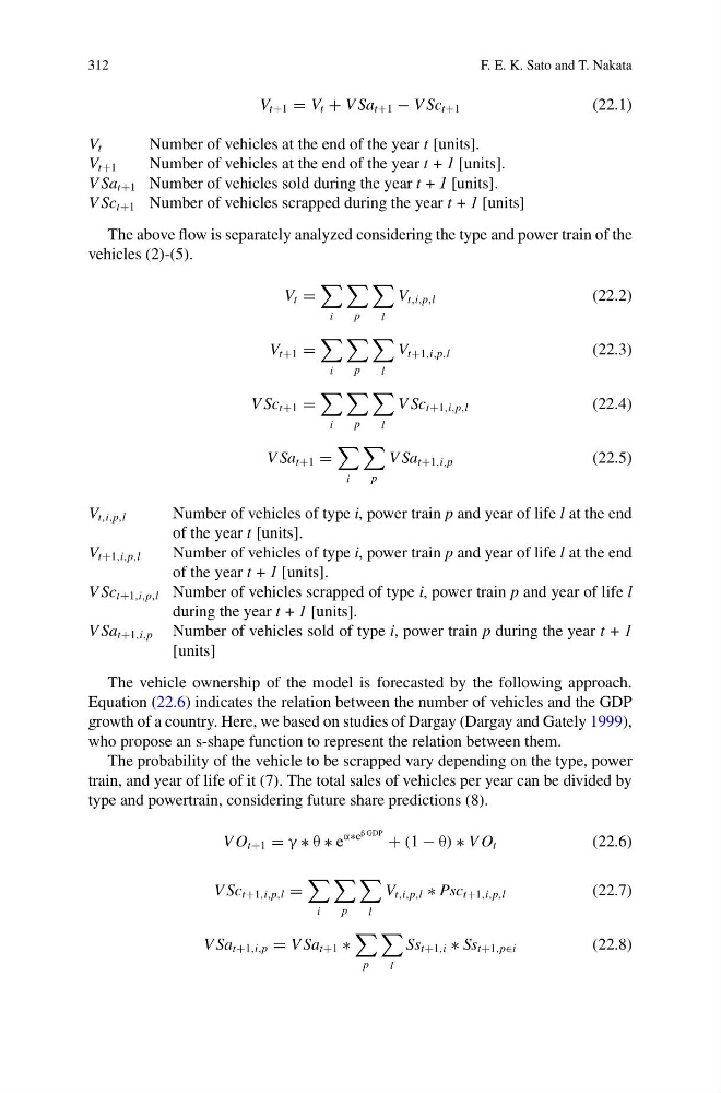
V t+1 = V t + V Sa t+1 − V Sc t+1
(22.1)
V t
Number of vehicles at the end of the year t [units].
V t+1
Number of vehicles at the end of the year t + 1 [units].
V Sa t+1 Number of vehicles sold during the year t + 1 [units].
V Sc t+1 Number of vehicles scrapped during the year t + 1 [units]
The above flow is separately analyzed considering the type and power train of the
vehicles (2)-(5).
V t =
i
p
l
V t,i,p,l
(22.2)
V t+1 =
i
p
l
V t+1,i,p,l
(22.3)
V Sc t+1 =
i
p
l
V Sc t+1,i,p,l
(22.4)
V Sa t+1 =
i
p
V Sa t+1,i,p
(22.5)
V t,i,p,l
Number of vehicles of type i, power train p and year of life l at the end
of the year t [units].
V t+1,i,p,l
Number of vehicles of type i, power train p and year of life l at the end
of the year t + 1 [units].
V Sc t+1,i,p,l Number of vehicles scrapped of type i, power train p and year of life l
during the year t + 1 [units].
V Sa t+1,i,p Number of vehicles sold of type i, power train p during the year t + 1
[units]
The vehicle ownership of the model is forecasted by the following approach.
Equation (22.6) indicates the relation between the number of vehicles and the GDP
growth of a country. Here, we based on studies of Dargay (Dargay and Gately 1999),
who propose an s-shape function to represent the relation between them.
The probability of the vehicle to be scrapped vary depending on the type, power
train, and year of life of it (7). The total sales of vehicles per year can be divided by
type and powertrain, considering future share predictions (8).
V O t+1 = γ ∗ θ ∗ e
α∗e
β GDP + (1 − θ) ∗ V O t
(22.6)
V Sc t+1,i,p,l =
i
p
l
V t,i,p,l ∗ Psc t+1,i,p,l
(22.7)
V Sa t+1,i,p = V Sa t+1 ∗
p
l
Ss t+1,i ∗ Ss t+1,p∈i
(22.8)
F. E. K. Sato and T. Nakata
V t+1 = V t + V Sa t+1 − V Sc t+1
(22.1)
V t
Number of vehicles at the end of the year t [units].
V t+1
Number of vehicles at the end of the year t + 1 [units].
V Sa t+1 Number of vehicles sold during the year t + 1 [units].
V Sc t+1 Number of vehicles scrapped during the year t + 1 [units]
The above flow is separately analyzed considering the type and power train of the
vehicles (2)-(5).
V t =
i
p
l
V t,i,p,l
(22.2)
V t+1 =
i
p
l
V t+1,i,p,l
(22.3)
V Sc t+1 =
i
p
l
V Sc t+1,i,p,l
(22.4)
V Sa t+1 =
i
p
V Sa t+1,i,p
(22.5)
V t,i,p,l
Number of vehicles of type i, power train p and year of life l at the end
of the year t [units].
V t+1,i,p,l
Number of vehicles of type i, power train p and year of life l at the end
of the year t + 1 [units].
V Sc t+1,i,p,l Number of vehicles scrapped of type i, power train p and year of life l
during the year t + 1 [units].
V Sa t+1,i,p Number of vehicles sold of type i, power train p during the year t + 1
[units]
The vehicle ownership of the model is forecasted by the following approach.
Equation (22.6) indicates the relation between the number of vehicles and the GDP
growth of a country. Here, we based on studies of Dargay (Dargay and Gately 1999),
who propose an s-shape function to represent the relation between them.
The probability of the vehicle to be scrapped vary depending on the type, power
train, and year of life of it (7). The total sales of vehicles per year can be divided by
type and powertrain, considering future share predictions (8).
V O t+1 = γ ∗ θ ∗ e
α∗e
β GDP + (1 − θ) ∗ V O t
(22.6)
V Sc t+1,i,p,l =
i
p
l
V t,i,p,l ∗ Psc t+1,i,p,l
(22.7)
V Sa t+1,i,p = V Sa t+1 ∗
p
l
Ss t+1,i ∗ Ss t+1,p∈i
(22.8)