

Modeling
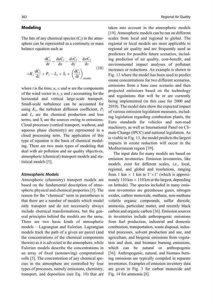
The fate of any chemical species (C i ) in the atmosphere can be represented as a continuity or mass
balance equation such as
dC i
dt
¼
duC i
dx
À
dvC i
dy
À
dwC i
dz
þK z
dC i
dz
þ P i À L i þ S i þ
dC i
dt
clouds
ð10Þ
where t is the time, u, v, and w are the components
of the wind vector in x, y, and z accounting for the
horizontal and vertical large-scale transport.
Small-scale turbulence can be accounted for
using K z , the turbulent diffusion coefficient, P i
and L i are the chemical production and loss
terms, and S i are the sources owing to emissions.
Cloud processes (vertical transport, washout, and
aqueous phase chemistry) are represented in a
cloud processing term. The application of this
type of equation is the basis of chemical modeling. There are two main types of modeling that
deal with air pollution and air quality objectives,
atmospheric (chemical) transport models and statistical models [5].
Atmospheric Models
Atmospheric (chemistry) transport models are
based on the fundamental description of atmospheric physical and chemical properties [5]. The
reason for the “chemical” term in parentheses is
that there are a number of models which model
only transport and do not necessarily always
include chemical transformations, but the general principles behind the models are the same.
There are two basic kinds of atmospheric
models – Lagrangian and Eulerian. Lagrangian
models track the path of a given air parcel (and
the concentrations of the chemical components
therein) as it is advected in the atmosphere, while
Eulerian models describe the concentrations in
an array of fixed (nonmoving) computational
cells [5]. The concentration of any chemical species in the atmosphere are controlled by four
types of processes, namely emissions, chemistry,
transport, and deposition (see Eq. 10) that are
taken into account in the atmospheric models
[19]. Atmospheric models can be run on different
scales from local and regional to global. The
regional or local models are most applicable to
regional air quality and are frequently used as
predictors for possible future scenarios, including prediction of air quality, cost-benefit, and
environmental impact analyses of pollutant
increases or reductions. An example is shown in
Fig. 13 where the model has been used to predict
ozone concentrations for two different scenarios,
emissions from a base case scenario and then
projected emissions based on the technology
and regulations that will be or are currently
being implemented (in this case for 2000 and
2010). The model data show the expected impact
of various emission legislation measures, including legislation regarding combustion plants, the
Euro standards for vehicles and non-road
machinery, as well as International Panel on Climate Change (IPCC) and national legislation. As
is visible in Fig. 13, the model predicts the largest
impacts in ozone reduction will occur in the
Mediterranean region [39].
The input data for many models are based on
emission inventories. Emission inventories, like
models, exist for different scales, i.e., local,
regional, and global and resolutions, ranging
from 1 km  1 km to 1
Â1
(which is approximately 110 km  110 km at the largest, depending
on latitude). The species included in many emission inventories are greenhouse gases, nitrogen
oxides, carbon monoxide, methane, non-methane
volatile organic compounds, sulfur dioxide,
ammonia, particulate matter, and recently black
carbon and organic carbon [36]. Emission sources
in inventories include anthropogenic emissions
from fuel production, industrial and domestic
combustion, transportation, waste disposal, industrial processes, solvent production and use, and
agriculture, and biogenic emissions from vegetation and dust, and biomass burning emissions,
which can be natural or anthropogenic
[36]. Anthropogenic, natural, and biomass burning emissions are typically compiled in separate
inventories. Examples of emission inventory data
are given in Fig. 3 for carbon monoxide and
Fig. 14 for ammonia [8].
362
Regional Air Quality
The fate of any chemical species (C i ) in the atmosphere can be represented as a continuity or mass
balance equation such as
dC i
dt
¼
duC i
dx
À
dvC i
dy
À
dwC i
dz
þK z
dC i
dz
þ P i À L i þ S i þ
dC i
dt
clouds
ð10Þ
where t is the time, u, v, and w are the components
of the wind vector in x, y, and z accounting for the
horizontal and vertical large-scale transport.
Small-scale turbulence can be accounted for
using K z , the turbulent diffusion coefficient, P i
and L i are the chemical production and loss
terms, and S i are the sources owing to emissions.
Cloud processes (vertical transport, washout, and
aqueous phase chemistry) are represented in a
cloud processing term. The application of this
type of equation is the basis of chemical modeling. There are two main types of modeling that
deal with air pollution and air quality objectives,
atmospheric (chemical) transport models and statistical models [5].
Atmospheric Models
Atmospheric (chemistry) transport models are
based on the fundamental description of atmospheric physical and chemical properties [5]. The
reason for the “chemical” term in parentheses is
that there are a number of models which model
only transport and do not necessarily always
include chemical transformations, but the general principles behind the models are the same.
There are two basic kinds of atmospheric
models – Lagrangian and Eulerian. Lagrangian
models track the path of a given air parcel (and
the concentrations of the chemical components
therein) as it is advected in the atmosphere, while
Eulerian models describe the concentrations in
an array of fixed (nonmoving) computational
cells [5]. The concentration of any chemical species in the atmosphere are controlled by four
types of processes, namely emissions, chemistry,
transport, and deposition (see Eq. 10) that are
taken into account in the atmospheric models
[19]. Atmospheric models can be run on different
scales from local and regional to global. The
regional or local models are most applicable to
regional air quality and are frequently used as
predictors for possible future scenarios, including prediction of air quality, cost-benefit, and
environmental impact analyses of pollutant
increases or reductions. An example is shown in
Fig. 13 where the model has been used to predict
ozone concentrations for two different scenarios,
emissions from a base case scenario and then
projected emissions based on the technology
and regulations that will be or are currently
being implemented (in this case for 2000 and
2010). The model data show the expected impact
of various emission legislation measures, including legislation regarding combustion plants, the
Euro standards for vehicles and non-road
machinery, as well as International Panel on Climate Change (IPCC) and national legislation. As
is visible in Fig. 13, the model predicts the largest
impacts in ozone reduction will occur in the
Mediterranean region [39].
The input data for many models are based on
emission inventories. Emission inventories, like
models, exist for different scales, i.e., local,
regional, and global and resolutions, ranging
from 1 km  1 km to 1
Â1
(which is approximately 110 km  110 km at the largest, depending
on latitude). The species included in many emission inventories are greenhouse gases, nitrogen
oxides, carbon monoxide, methane, non-methane
volatile organic compounds, sulfur dioxide,
ammonia, particulate matter, and recently black
carbon and organic carbon [36]. Emission sources
in inventories include anthropogenic emissions
from fuel production, industrial and domestic
combustion, transportation, waste disposal, industrial processes, solvent production and use, and
agriculture, and biogenic emissions from vegetation and dust, and biomass burning emissions,
which can be natural or anthropogenic
[36]. Anthropogenic, natural, and biomass burning emissions are typically compiled in separate
inventories. Examples of emission inventory data
are given in Fig. 3 for carbon monoxide and
Fig. 14 for ammonia [8].
362
Regional Air Quality