

boundary layer (e.g., Molina and Molina [7]). In
other locations, regional weather patterns lead to
persistent patterns of pollutant exposure, for
example, the daily sea breeze circulation affecting Hong Kong and the Pearl River Delta
[8]. Local circulation patterns and topography
can therefore exacerbate, or ameliorate, the
atmospheric composition resulting from a given
emissions situation [9]; and the combined effects
of local and regional scale dynamics, mixing and
chemical transformations must be considered in
the development of urban air quality management policies.
Basic Composition and Key Pollutants
The bulk atmospheric composition is essentially
constant throughout the troposphere, comprising
gases such as nitrogen, oxygen, argon, helium,
carbon dioxide and a variable amount of water
vapor. Most concern over urban atmospheric
composition and air pollution arises from the
trace components – gaseous constituents such as
ozone, nitrogen oxides and volatile organic compounds, and suspended particulate material
(PM) commonly referred to as aerosol (although
strictly the term denotes both the condensed phase
material and the gas it is suspended within).
Urban air pollution issues primarily relate to local
emissions and the chemical processing of pollutants
and natural atmospheric species which occurs on
timescales of a few hours to a few days. This can
be distinguished from the wider, regional impacts of
air pollution (such as increasing background ozone
levels, and the abundance of sulfate aerosol),
although these also impact on the urban environment and are considered here. Global air pollution
issues related to long-lived species such as CFC,
HCFC and halon compounds contributing to stratospheric ozone depletion, and the climate-related
issues associated with the global abundance of
longer-lived greenhouse gases such as carbon dioxide and methane, are not discussed further here –
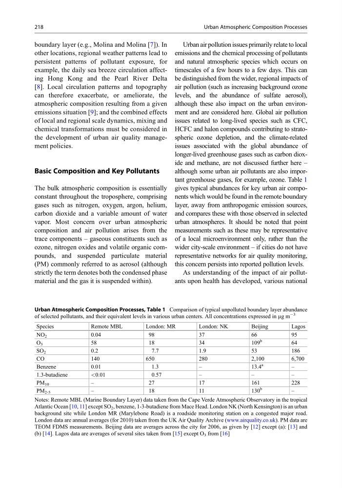
although some urban air pollutants are also important greenhouse gases, for example, ozone. Table 1
gives typical abundances for key urban air components which would be found in the remote boundary
layer, away from anthropogenic emission sources,
and compares these with those observed in selected
urban atmospheres. It should be noted that point
measurements such as these may be representative
of a local microenvironment only, rather than the
wider city-scale environment – if cities do not have
representative networks for air quality monitoring,
this concern persists into reported pollution levels.
As understanding of the impact of air pollutants upon health has developed, various national
Urban Atmospheric Composition Processes, Table 1 Comparison of typical unpolluted boundary layer abundance
of selected pollutants, and their equivalent levels in various urban centers. All concentrations expressed in mg m
À3
Species
Remote MBL
London: MR
London: NK
Beijing
Lagos
NO 2
0.04
98
37
66
95
O 3
58
18
34
109
b
64
SO 2
0.2
7.7
1.9
53
186
CO
140
650
280
2,100
6,700
Benzene
0.01
1.3
–
13.4
a
–
1.3-butadiene
<0.01
0.57
–
–
–
PM 10
–
27
17
161
228
PM 2 . 5
–
18
11
130
b
–
Notes: Remote MBL (Marine Boundary Layer) data taken from the Cape Verde Atmospheric Observatory in the tropical
Atlantic Ocean [10, 11] except SO 2 , benzene, 1-3-butadiene from Mace Head. London NK (North Kensington) is an urban
background site while London MR (Marylebone Road) is a roadside monitoring station on a congested major road.
London data are annual averages (for 2010) taken from the UK Air Quality Archive (www.airquality.co.uk). PM data are
TEOM FDMS measurements. Beijing data are averages across the city for 2006, as given by [12] except (a): [13] and
(b) [14]. Lagos data are averages of several sites taken from [15] except O 3 from [16]
218
Urban Atmospheric Composition Processes
other locations, regional weather patterns lead to
persistent patterns of pollutant exposure, for
example, the daily sea breeze circulation affecting Hong Kong and the Pearl River Delta
[8]. Local circulation patterns and topography
can therefore exacerbate, or ameliorate, the
atmospheric composition resulting from a given
emissions situation [9]; and the combined effects
of local and regional scale dynamics, mixing and
chemical transformations must be considered in
the development of urban air quality management policies.
Basic Composition and Key Pollutants
The bulk atmospheric composition is essentially
constant throughout the troposphere, comprising
gases such as nitrogen, oxygen, argon, helium,
carbon dioxide and a variable amount of water
vapor. Most concern over urban atmospheric
composition and air pollution arises from the
trace components – gaseous constituents such as
ozone, nitrogen oxides and volatile organic compounds, and suspended particulate material
(PM) commonly referred to as aerosol (although
strictly the term denotes both the condensed phase
material and the gas it is suspended within).
Urban air pollution issues primarily relate to local
emissions and the chemical processing of pollutants
and natural atmospheric species which occurs on
timescales of a few hours to a few days. This can
be distinguished from the wider, regional impacts of
air pollution (such as increasing background ozone
levels, and the abundance of sulfate aerosol),
although these also impact on the urban environment and are considered here. Global air pollution
issues related to long-lived species such as CFC,
HCFC and halon compounds contributing to stratospheric ozone depletion, and the climate-related
issues associated with the global abundance of
longer-lived greenhouse gases such as carbon dioxide and methane, are not discussed further here –
although some urban air pollutants are also important greenhouse gases, for example, ozone. Table 1
gives typical abundances for key urban air components which would be found in the remote boundary
layer, away from anthropogenic emission sources,
and compares these with those observed in selected
urban atmospheres. It should be noted that point
measurements such as these may be representative
of a local microenvironment only, rather than the
wider city-scale environment – if cities do not have
representative networks for air quality monitoring,
this concern persists into reported pollution levels.
As understanding of the impact of air pollutants upon health has developed, various national
Urban Atmospheric Composition Processes, Table 1 Comparison of typical unpolluted boundary layer abundance
of selected pollutants, and their equivalent levels in various urban centers. All concentrations expressed in mg m
À3
Species
Remote MBL
London: MR
London: NK
Beijing
Lagos
NO 2
0.04
98
37
66
95
O 3
58
18
34
109
b
64
SO 2
0.2
7.7
1.9
53
186
CO
140
650
280
2,100
6,700
Benzene
0.01
1.3
–
13.4
a
–
1.3-butadiene
<0.01
0.57
–
–
–
PM 10
–
27
17
161
228
PM 2 . 5
–
18
11
130
b
–
Notes: Remote MBL (Marine Boundary Layer) data taken from the Cape Verde Atmospheric Observatory in the tropical
Atlantic Ocean [10, 11] except SO 2 , benzene, 1-3-butadiene from Mace Head. London NK (North Kensington) is an urban
background site while London MR (Marylebone Road) is a roadside monitoring station on a congested major road.
London data are annual averages (for 2010) taken from the UK Air Quality Archive (www.airquality.co.uk). PM data are
TEOM FDMS measurements. Beijing data are averages across the city for 2006, as given by [12] except (a): [13] and
(b) [14]. Lagos data are averages of several sites taken from [15] except O 3 from [16]
218
Urban Atmospheric Composition Processes