

in the street canyon. CFD results agree well with
wind tunnel measurements.
It is known that FCM type of models still
suffers from their high computational cost which
prevents them from being largely employed in
operational applications. This has pushed the
development of FAM models yet incorporating
new understanding of flow and dispersion processes within the urban canopy layer. Recently,
di Sabatino et al. [82] have proposed a new modelling approach for the computation of the spatiallyaveraged flow field, where the average is defined
at the neighborhood scale, i.e., from 0.2 km up to
10 km. The underlying idea is the description of
the drag forces in terms of height-dependent morphological parameters based on detailed knowledge of building geometry such as the planar area
index l p and l f (introduced in section “Characteristic Regions of the Flow and Drivers”) and the
reduction of the complete three-dimensional flow
field to a one-dimensional quantity, given by the
mean wind direction, and the three-dimensional
spatial dependence to a much more simple dependence from the height z. As a consequence, only
mean profiles are needed as input to the model.
There are examples in the literature [83] showing
the possibility of extending this modelling
approach to an Eulerian dispersion model for the
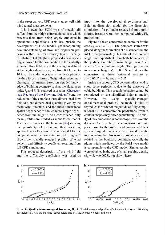
computation of the concentration field. Figure 7
shows the spatially-averaged profiles of wind
velocity and diffusivity coefficient resulting from
full CFD simulations.
This reduced description of the wind field
and the diffusivity coefficient was used as
input into the developed three-dimensional
Eulerian dispersion model for the dispersion
simulation of a pollutant released from a point
source. Results were then compared with CFD
predictions.
Figure 8 shows concentration contours for the
case l p ¼ l f ¼ 0.16. The pollutant source was
placed along the x direction at a distance from the
inlet of approximately 1/3–1/4 of the domain
length and equidistant from both boundaries in
the y direction. The domain height was 6 H,
where H is the building height. The figure refers
to a source height Z s ¼ 0.5 H and shows the
comparison at three horizontal sections at
z ¼ 0.05 H, z ¼ H, and z ¼ 2 H.
Inside the canopy, CFD concentrations tend to
show some periodicity, due to the presence of
cubic buildings. This specific behavior cannot be
reproduced by the simplified Eulerian model.
However,
by
using
spatially-averaged
one-dimensional profiles, the model is able to
reproduce the order of magnitude of fully computational CFD concentration predictions, even if
contour shapes may differ qualitatively. The quality of the comparison is not homogeneous over the
domain. As expected, the comparison is quite
poor close to the source and improves downstream. Large differences are also found near the
top boundary, but this is most probably an effect
related to the boundary condition. Overall, the
plume width predicted by the FAM type model
is comparable to the CFD model. Similar results
were obtained in the case of small packing density
(l p ¼ l f ¼ 0.0625), not shown here.
0
a
0
1
2
z/H
3
4
5
λ p = 0.0625
λ p = 0.16
6
1.1
1
0.9
0.8
0.7
0.6
U/U ref
0.5
0.4
0.3
0.2
5
2
0
.
0
2
0
.
0
5
1
0
.
0
1
0
.
0
5
0
0
.
0
0
1
.
0
0
1
2
z/H
3
4
5
λ p = 0.0625
λ p = 0.16
6
0.03
D/(U ref H)
b
Urban Air Quality: Meteorological Processes, Fig. 7 Spatially-averaged profiles of wind velocity (a) and diffusivity
coefficient (b). H is the building (cube) height and U ref the average velocity at the top
Urban Air Quality: Meteorological Processes
185
wind tunnel measurements.
It is known that FCM type of models still
suffers from their high computational cost which
prevents them from being largely employed in
operational applications. This has pushed the
development of FAM models yet incorporating
new understanding of flow and dispersion processes within the urban canopy layer. Recently,
di Sabatino et al. [82] have proposed a new modelling approach for the computation of the spatiallyaveraged flow field, where the average is defined
at the neighborhood scale, i.e., from 0.2 km up to
10 km. The underlying idea is the description of
the drag forces in terms of height-dependent morphological parameters based on detailed knowledge of building geometry such as the planar area
index l p and l f (introduced in section “Characteristic Regions of the Flow and Drivers”) and the
reduction of the complete three-dimensional flow
field to a one-dimensional quantity, given by the
mean wind direction, and the three-dimensional
spatial dependence to a much more simple dependence from the height z. As a consequence, only
mean profiles are needed as input to the model.
There are examples in the literature [83] showing
the possibility of extending this modelling
approach to an Eulerian dispersion model for the
computation of the concentration field. Figure 7
shows the spatially-averaged profiles of wind
velocity and diffusivity coefficient resulting from
full CFD simulations.
This reduced description of the wind field
and the diffusivity coefficient was used as
input into the developed three-dimensional
Eulerian dispersion model for the dispersion
simulation of a pollutant released from a point
source. Results were then compared with CFD
predictions.
Figure 8 shows concentration contours for the
case l p ¼ l f ¼ 0.16. The pollutant source was
placed along the x direction at a distance from the
inlet of approximately 1/3–1/4 of the domain
length and equidistant from both boundaries in
the y direction. The domain height was 6 H,
where H is the building height. The figure refers
to a source height Z s ¼ 0.5 H and shows the
comparison at three horizontal sections at
z ¼ 0.05 H, z ¼ H, and z ¼ 2 H.
Inside the canopy, CFD concentrations tend to
show some periodicity, due to the presence of
cubic buildings. This specific behavior cannot be
reproduced by the simplified Eulerian model.
However,
by
using
spatially-averaged
one-dimensional profiles, the model is able to
reproduce the order of magnitude of fully computational CFD concentration predictions, even if
contour shapes may differ qualitatively. The quality of the comparison is not homogeneous over the
domain. As expected, the comparison is quite
poor close to the source and improves downstream. Large differences are also found near the
top boundary, but this is most probably an effect
related to the boundary condition. Overall, the
plume width predicted by the FAM type model
is comparable to the CFD model. Similar results
were obtained in the case of small packing density
(l p ¼ l f ¼ 0.0625), not shown here.
0
a
0
1
2
z/H
3
4
5
λ p = 0.0625
λ p = 0.16
6
1.1
1
0.9
0.8
0.7
0.6
U/U ref
0.5
0.4
0.3
0.2
5
2
0
.
0
2
0
.
0
5
1
0
.
0
1
0
.
0
5
0
0
.
0
0
1
.
0
0
1
2
z/H
3
4
5
λ p = 0.0625
λ p = 0.16
6
0.03
D/(U ref H)
b
Urban Air Quality: Meteorological Processes, Fig. 7 Spatially-averaged profiles of wind velocity (a) and diffusivity
coefficient (b). H is the building (cube) height and U ref the average velocity at the top
Urban Air Quality: Meteorological Processes
185