

to increase charging of aerosol particles so they
can be removed using electrostatic force. ESPs
can also be operated in negative mode. The electrode is given a large negative charge and emits
electrons that attach to particles. Two main types
of collection electrodes are used in ESPs: flat
plates and tubes (Fig. 11b). The typical space
between the electrodes and the plates is
10–15 cm. Particles are separated from the gas
stream as it passes between them (Fig. 11a)
resulting in the formation of a particulate cake
on the plates. Some systems include shakers or
hammers to clean the plates. In the tubular configuration, which is more common for wet ESPs,
the discharge electrode is located at the center of a
tubular collector electrode. The diameter of tubes
can be 8–25 cm with a 1–4 m length (Fig. 11b). In
this design, the discharge electrode is parallel to
the gas flow [5, 70].
An electrical potential of ~4 kV/cm is used to
create the corona discharge, applied between the
discharge and collection electrodes. Generally, the
wires are charged at 20–100 kV below ground
potential. In most cases a negative corona
(Fig. 11c) is more stable than a positive corona;
however, negative corona plasmas also produce
much more ozone which can be an unwanted
byproduct. Negative coronas are typically chosen
because their stability leads to better performance
(e.g., less arcing) and lower cost.
In a negative mode operation, negative ions fill
the space outside the corona and then collide with
particles, charging them negatively (Fig. 11d).
The charged particles are driven onto the positive
collector plates by an electrical field. Electrostatic
charging of particles occurs via two mechanisms,
bombardment charging (important for micronsized particles) and diffusion charging
(important for submicron particles). When the
initial distribution has relaxed to equilibrium, the
charge on the particles will be proportional to
particle surface area, i.e., d p
2 . As submicron particles (<0.1 mm) have significant diffusional
motion, they will be charged significantly by diffusional charging. Thus, ESPs are widely used to
control submicron particles.
Table 6 shows many advantages and disadvantages of ESP technologies used to control
particles.
ESP Performance
Deutsch equation is a common description of
particle collection efficiency (E) for monodisperse
particles:
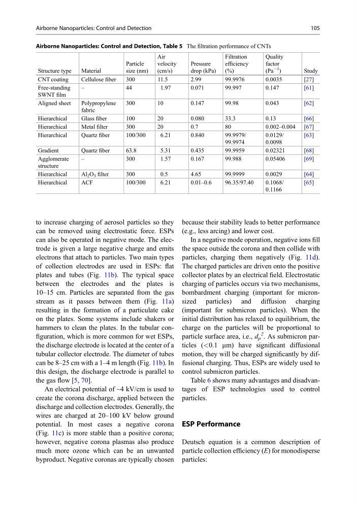
Airborne Nanoparticles: Control and Detection, Table 5 The filtration performance of CNTs
Structure type
Material
Particle
size (nm)
Air
velocity
(cm/s)
Pressure
drop (kPa)
Filtration
efficiency
(%)
Quality
factor
(Pa
À1
)
Study
CNT coating
Cellulose fiber
300
11.5
2.99
99.9976
0.0035
[27]
Free-standing
SWNT film
–
44
1.97
0.071
99.997
0.147
[61]
Aligned sheet
Polypropylene
fabric
300
10
0.147
99.98
0.043
[62]
Hierarchical
Glass fiber
100
20
0.080
33.3
0.13
[66]
Hierarchical
Metal filter
300
20
0.7
80
0.002–0.004 [67]
Hierarchical
Quartz fiber
100/300
6.21
0.840
99.9979/
99.9974
0.0129/
0.0098
[63]
Gradient
Quartz fiber
63.8
5.31
0.435
99.9959
0.02321
[68]
Agglomerate
structure
–
300
1.57
0.167
99.988
0.05406
[69]
Hierarchical
Al 2 O 3 filter
300
0.5
4.65
99.9999
0.0029
[64]
Hierarchical
ACF
100/300
6.21
0.01–0.6
96.35/97.40
0.1068/
0.1166
[65]
Airborne Nanoparticles: Control and Detection
105
can be removed using electrostatic force. ESPs
can also be operated in negative mode. The electrode is given a large negative charge and emits
electrons that attach to particles. Two main types
of collection electrodes are used in ESPs: flat
plates and tubes (Fig. 11b). The typical space
between the electrodes and the plates is
10–15 cm. Particles are separated from the gas
stream as it passes between them (Fig. 11a)
resulting in the formation of a particulate cake
on the plates. Some systems include shakers or
hammers to clean the plates. In the tubular configuration, which is more common for wet ESPs,
the discharge electrode is located at the center of a
tubular collector electrode. The diameter of tubes
can be 8–25 cm with a 1–4 m length (Fig. 11b). In
this design, the discharge electrode is parallel to
the gas flow [5, 70].
An electrical potential of ~4 kV/cm is used to
create the corona discharge, applied between the
discharge and collection electrodes. Generally, the
wires are charged at 20–100 kV below ground
potential. In most cases a negative corona
(Fig. 11c) is more stable than a positive corona;
however, negative corona plasmas also produce
much more ozone which can be an unwanted
byproduct. Negative coronas are typically chosen
because their stability leads to better performance
(e.g., less arcing) and lower cost.
In a negative mode operation, negative ions fill
the space outside the corona and then collide with
particles, charging them negatively (Fig. 11d).
The charged particles are driven onto the positive
collector plates by an electrical field. Electrostatic
charging of particles occurs via two mechanisms,
bombardment charging (important for micronsized particles) and diffusion charging
(important for submicron particles). When the
initial distribution has relaxed to equilibrium, the
charge on the particles will be proportional to
particle surface area, i.e., d p
2 . As submicron particles (<0.1 mm) have significant diffusional
motion, they will be charged significantly by diffusional charging. Thus, ESPs are widely used to
control submicron particles.
Table 6 shows many advantages and disadvantages of ESP technologies used to control
particles.
ESP Performance
Deutsch equation is a common description of
particle collection efficiency (E) for monodisperse
particles:
Airborne Nanoparticles: Control and Detection, Table 5 The filtration performance of CNTs
Structure type
Material
Particle
size (nm)
Air
velocity
(cm/s)
Pressure
drop (kPa)
Filtration
efficiency
(%)
Quality
factor
(Pa
À1
)
Study
CNT coating
Cellulose fiber
300
11.5
2.99
99.9976
0.0035
[27]
Free-standing
SWNT film
–
44
1.97
0.071
99.997
0.147
[61]
Aligned sheet
Polypropylene
fabric
300
10
0.147
99.98
0.043
[62]
Hierarchical
Glass fiber
100
20
0.080
33.3
0.13
[66]
Hierarchical
Metal filter
300
20
0.7
80
0.002–0.004 [67]
Hierarchical
Quartz fiber
100/300
6.21
0.840
99.9979/
99.9974
0.0129/
0.0098
[63]
Gradient
Quartz fiber
63.8
5.31
0.435
99.9959
0.02321
[68]
Agglomerate
structure
–
300
1.57
0.167
99.988
0.05406
[69]
Hierarchical
Al 2 O 3 filter
300
0.5
4.65
99.9999
0.0029
[64]
Hierarchical
ACF
100/300
6.21
0.01–0.6
96.35/97.40
0.1068/
0.1166
[65]
Airborne Nanoparticles: Control and Detection
105