

2.4.7 Twiss functions and matrix formalism
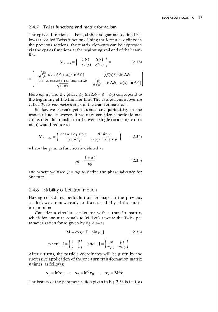
The optical functions — beta, alpha and gamma (defined below) are called Twiss functions. Using the formulas defined in
the previous sections, the matrix elements can be expressed
via the optics functions at the beginning and end of the beamline:
(
)
C(s)
S(s)
M s 0 →s =
=
(2.33)
−C ' (s) S ' (s)
⎛ )
⎞
.
β(s)
⎜
⎟
⎜
(cos Δφ + α 0 sin Δφ)
β(s)β 0 sin Δφ
⎟
⎜
⎟
⎜
β 0
⎟
⎜
)
⎟
= ⎜
⎟
⎜ ⎜ −
(α(s)−α 0 ) cos Δφ+(1+α(s)α 0 ) sin Δφ
β 0
⎟ ⎟
⎝
√
[cos Δφ − α(s) sin Δφ]⎠
β(s)
β(s)β 0
Here β 0 , α 0 and the phase φ 0 (in Δφ = φ − φ 0 ) correspond to
the beginning of the transfer line. The expressions above are
called Twiss parameterization of the transfer matrices.
So far, we haven’t yet assumed any periodicity in the
transfer line. However, if we now consider a periodic machine, then the transfer matrix over a single turn (single turn
map) would reduce to
(
)
cos μ + α 0 sin μ
β 0 sin μ
M s 0 →s 0 =
(2.34)
−γ 0 sin μ
cos μ − α 0 sin μ
where the gamma function is defined as
1 + α 0
2
γ 0 =
(2.35)
β 0
and where we used μ = Δφ to define the phase advance for
one turn.
2.4.8 Stability of betatron motion
Having considered periodic transfer maps in the previous
section, we are now ready to discuss stability of the multiturn motion.
Consider a circular accelerator with a transfer matrix,
which for one turn equals to M. Let’s rewrite the Twiss parameterization for M given by Eg.2.34 as
M = cos μ · I + sin μ · J
(2.36)
(
)
(
)
1 0
α 0
β 0
where I =
and J =
0 1
−γ 0 −α 0
After n turns, the particle coordinates will be given by the
successive application of the one-turn transformation matrix
n times, as follows:
x 1 = Mx 0 ... x 2 = M
2 x 0 ... x n = M
n x 0
The beauty of the parametrization given in Eq. 2.36 is that, as
transverse dynamics 33
The optical functions — beta, alpha and gamma (defined below) are called Twiss functions. Using the formulas defined in
the previous sections, the matrix elements can be expressed
via the optics functions at the beginning and end of the beamline:
(
)
C(s)
S(s)
M s 0 →s =
=
(2.33)
−C ' (s) S ' (s)
⎛ )
⎞
.
β(s)
⎜
⎟
⎜
(cos Δφ + α 0 sin Δφ)
β(s)β 0 sin Δφ
⎟
⎜
⎟
⎜
β 0
⎟
⎜
)
⎟
= ⎜
⎟
⎜ ⎜ −
(α(s)−α 0 ) cos Δφ+(1+α(s)α 0 ) sin Δφ
β 0
⎟ ⎟
⎝
√
[cos Δφ − α(s) sin Δφ]⎠
β(s)
β(s)β 0
Here β 0 , α 0 and the phase φ 0 (in Δφ = φ − φ 0 ) correspond to
the beginning of the transfer line. The expressions above are
called Twiss parameterization of the transfer matrices.
So far, we haven’t yet assumed any periodicity in the
transfer line. However, if we now consider a periodic machine, then the transfer matrix over a single turn (single turn
map) would reduce to
(
)
cos μ + α 0 sin μ
β 0 sin μ
M s 0 →s 0 =
(2.34)
−γ 0 sin μ
cos μ − α 0 sin μ
where the gamma function is defined as
1 + α 0
2
γ 0 =
(2.35)
β 0
and where we used μ = Δφ to define the phase advance for
one turn.
2.4.8 Stability of betatron motion
Having considered periodic transfer maps in the previous
section, we are now ready to discuss stability of the multiturn motion.
Consider a circular accelerator with a transfer matrix,
which for one turn equals to M. Let’s rewrite the Twiss parameterization for M given by Eg.2.34 as
M = cos μ · I + sin μ · J
(2.36)
(
)
(
)
1 0
α 0
β 0
where I =
and J =
0 1
−γ 0 −α 0
After n turns, the particle coordinates will be given by the
successive application of the one-turn transformation matrix
n times, as follows:
x 1 = Mx 0 ... x 2 = M
2 x 0 ... x n = M
n x 0
The beauty of the parametrization given in Eq. 2.36 is that, as
transverse dynamics 33