

advanced beam manipulation, cooling, damping and stability 207
into the beamline specifically for the purpose of enhancing
the tune spread and thus helping the beam stability.
We would like to mention here that increasing the spread
of tunes or energy often helps accelerators simply because
it enhances the decoherence, preventing particles from assembling into collective motion. The term Landau damping
is sometimes used in cases where the term decoherence would
be more appropriate. 7 Details of a particular physics setting
define which of those two mechanisms is acting in each situation.
10.3.5 Stability and spectral approach
Beam or laser pulse stability issues are often analyzed based
on a spectral approach. We will omit detailed and rigorous
definitions here and focus only on a few highlights.
The disturbance — e.g., the position of a particular magnetic lens or optical element of a laser (we will define it as
x(t)) — often has the same characteristics as a random process. In this case, the notion of the power spectral density p(f )
(dubbed “power spectrum”) should be used instead of the
usual Fourier spectrum.
The key property of the power spectrum is that its integral
is equal to the variance σ of the signal x:
+∞
σ
2 = (x
2
) =
p(f ) df
(10.23)
−∞
where we assume that the average of x is zero: (x) = 0.
Disturbance to our beam or laser line often comes from
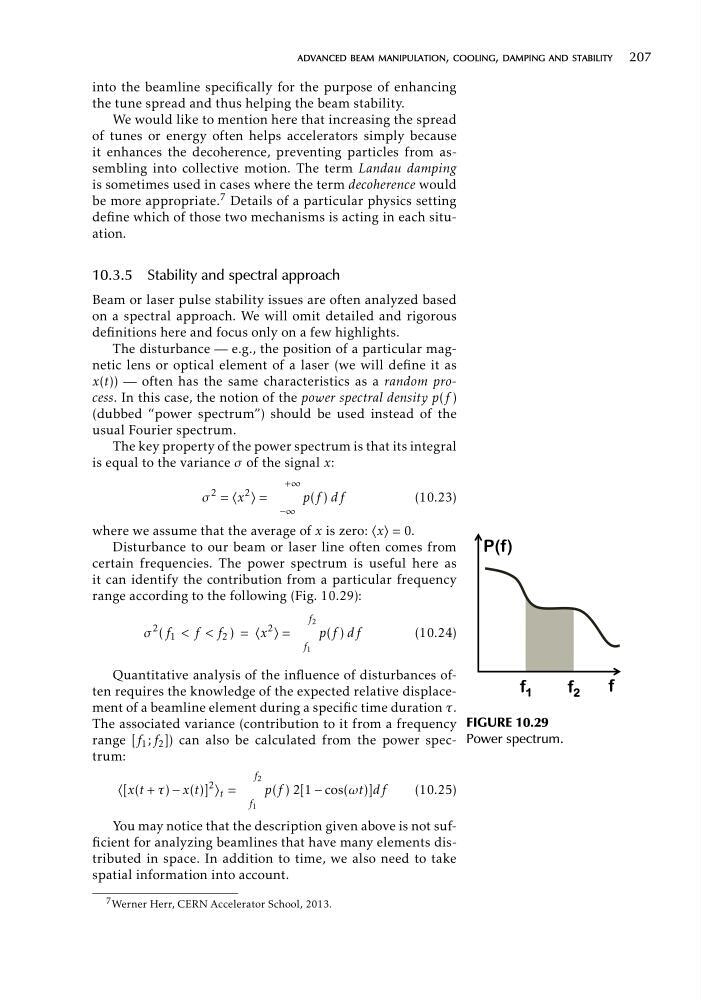
certain frequencies. The power spectrum is useful here as
it can identify the contribution from a particular frequency
range according to the following (Fig. 10.29):
f 2
2
2
σ ( f 1 < f < f 2 ) = (x ) =
p(f ) df
(10.24)
f 1
Quantitative analysis of the influence of disturbances often requires the knowledge of the expected relative displacement of a beamline element during a specific time duration τ.
The associated variance (contribution to it from a frequency FI
range [f 1 ; f 2 ]) can also be calculated from the power spec- P
trum:
f 2
([x(t + τ) − x(t)]
2
) t =
p(f ) 2[1 cos(ωt)]df
(10.25)
f 1
−
You may notice that the description given above is not sufficient for analyzing beamlines that have many elements distributed in space. In addition to time, we also need to take
spatial information into account.
7 Werner Herr, CERN Accelerator School, 2013.
GURE 10.29
ower spectrum.
3I
I
I
I
into the beamline specifically for the purpose of enhancing
the tune spread and thus helping the beam stability.
We would like to mention here that increasing the spread
of tunes or energy often helps accelerators simply because
it enhances the decoherence, preventing particles from assembling into collective motion. The term Landau damping
is sometimes used in cases where the term decoherence would
be more appropriate. 7 Details of a particular physics setting
define which of those two mechanisms is acting in each situation.
10.3.5 Stability and spectral approach
Beam or laser pulse stability issues are often analyzed based
on a spectral approach. We will omit detailed and rigorous
definitions here and focus only on a few highlights.
The disturbance — e.g., the position of a particular magnetic lens or optical element of a laser (we will define it as
x(t)) — often has the same characteristics as a random process. In this case, the notion of the power spectral density p(f )
(dubbed “power spectrum”) should be used instead of the
usual Fourier spectrum.
The key property of the power spectrum is that its integral
is equal to the variance σ of the signal x:
+∞
σ
2 = (x
2
) =
p(f ) df
(10.23)
−∞
where we assume that the average of x is zero: (x) = 0.
Disturbance to our beam or laser line often comes from
certain frequencies. The power spectrum is useful here as
it can identify the contribution from a particular frequency
range according to the following (Fig. 10.29):
f 2
2
2
σ ( f 1 < f < f 2 ) = (x ) =
p(f ) df
(10.24)
f 1
Quantitative analysis of the influence of disturbances often requires the knowledge of the expected relative displacement of a beamline element during a specific time duration τ.
The associated variance (contribution to it from a frequency FI
range [f 1 ; f 2 ]) can also be calculated from the power spec- P
trum:
f 2
([x(t + τ) − x(t)]
2
) t =
p(f ) 2[1 cos(ωt)]df
(10.25)
f 1
−
You may notice that the description given above is not sufficient for analyzing beamlines that have many elements distributed in space. In addition to time, we also need to take
spatial information into account.
7 Werner Herr, CERN Accelerator School, 2013.
GURE 10.29
ower spectrum.
3I
I
I
I