

advanced beam manipulation, cooling, damping and stability 187
on a straighter path through the chicane, catching up with the
synchronous particle, and resulting in bunch compression.
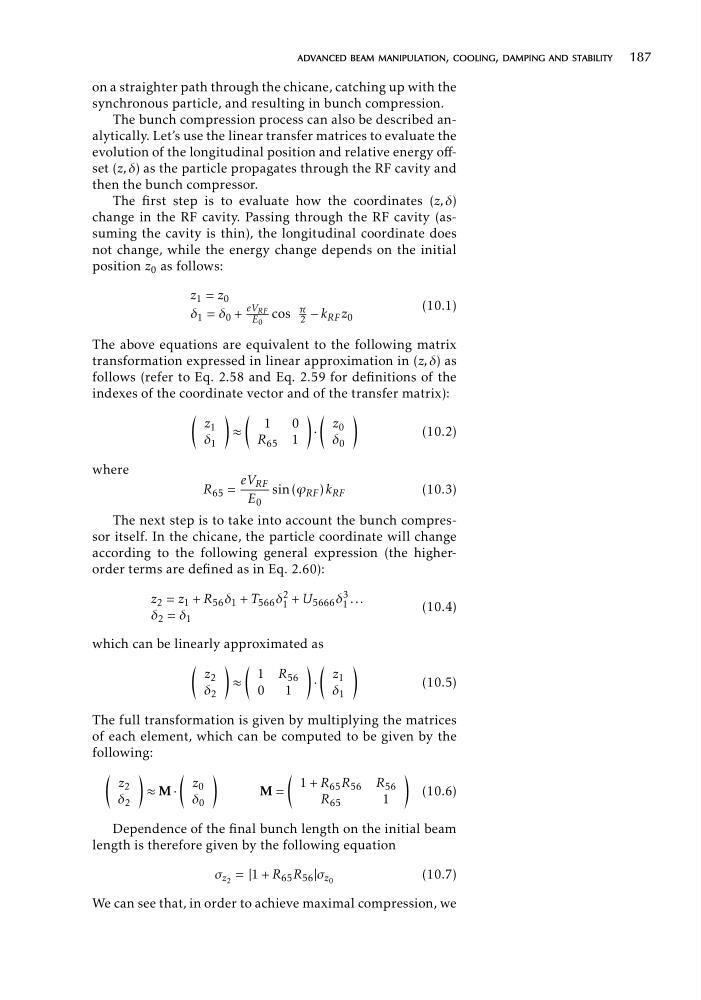
The bunch compression process can also be described analytically. Let’s use the linear transfer matrices to evaluate the
evolution of the longitudinal position and relative energy offset (z, δ) as the particle propagates through the RF cavity and
then the bunch compressor.
The first step is to evaluate how the coordinates (z, δ)
change in the RF cavity. Passing through the RF cavity (assuming the cavity is thin), the longitudinal coordinate does
not change, while the energy change depends on the initial
position z 0 as follows:
z 1 = z 0
= δ 0 +
eV RF
π
(10.1)
δ 1
E 0
cos 2 − k RF z 0
The above equations are equivalent to the following matrix
transformation expressed in linear approximation in (z, δ) as
follows (refer to Eq. 2.58 and Eq. 2.59 for definitions of the
indexes of the coordinate vector and of the transfer matrix):
(
) (
) (
)
z 1
1
0
z 0
≈
·
(10.2)
δ 1
R 65 1
δ 0
where
eV RF
R 65 =
sin (ϕ RF ) k RF
(10.3)
E 0
The next step is to take into account the bunch compressor itself. In the chicane, the particle coordinate will change
according to the following general expression (the higherorder terms are defined as in Eq. 2.60):
1 ...
z 2 = z 1 + R 56 δ 1 + T 566 δ 1
2 + U 5666 δ
3
(10.4)
δ 2 = δ 1
which can be linearly approximated as
(
) (
) (
)
z 2
1 R 56
z 1
≈
·
(10.5)
δ 2
0
1
δ 1
The full transformation is given by multiplying the matrices
of each element, which can be computed to be given by the
following:
(
)
(
)
(
)
z 2
z 0
1 + R 65 R 56 R 56
≈ M ·
M =
(10.6)
δ 2
δ 0
R 65
1
Dependence of the final bunch length on the initial beam
length is therefore given by the following equation
σ z 2 = |1 + R 65 R 56 |σ z 0
(10.7)
We can see that, in order to achieve maximal compression, we
on a straighter path through the chicane, catching up with the
synchronous particle, and resulting in bunch compression.
The bunch compression process can also be described analytically. Let’s use the linear transfer matrices to evaluate the
evolution of the longitudinal position and relative energy offset (z, δ) as the particle propagates through the RF cavity and
then the bunch compressor.
The first step is to evaluate how the coordinates (z, δ)
change in the RF cavity. Passing through the RF cavity (assuming the cavity is thin), the longitudinal coordinate does
not change, while the energy change depends on the initial
position z 0 as follows:
z 1 = z 0
= δ 0 +
eV RF
π
(10.1)
δ 1
E 0
cos 2 − k RF z 0
The above equations are equivalent to the following matrix
transformation expressed in linear approximation in (z, δ) as
follows (refer to Eq. 2.58 and Eq. 2.59 for definitions of the
indexes of the coordinate vector and of the transfer matrix):
(
) (
) (
)
z 1
1
0
z 0
≈
·
(10.2)
δ 1
R 65 1
δ 0
where
eV RF
R 65 =
sin (ϕ RF ) k RF
(10.3)
E 0
The next step is to take into account the bunch compressor itself. In the chicane, the particle coordinate will change
according to the following general expression (the higherorder terms are defined as in Eq. 2.60):
1 ...
z 2 = z 1 + R 56 δ 1 + T 566 δ 1
2 + U 5666 δ
3
(10.4)
δ 2 = δ 1
which can be linearly approximated as
(
) (
) (
)
z 2
1 R 56
z 1
≈
·
(10.5)
δ 2
0
1
δ 1
The full transformation is given by multiplying the matrices
of each element, which can be computed to be given by the
following:
(
)
(
)
(
)
z 2
z 0
1 + R 65 R 56 R 56
≈ M ·
M =
(10.6)
δ 2
δ 0
R 65
1
Dependence of the final bunch length on the initial beam
length is therefore given by the following equation
σ z 2 = |1 + R 65 R 56 |σ z 0
(10.7)
We can see that, in order to achieve maximal compression, we