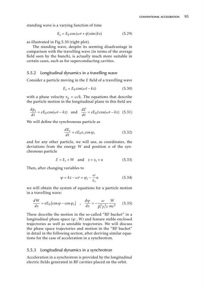
standing wave is a varying function of time
E z = E 0 cos (ωt + φ) sin (kz)
(5.29)
as illustrated in Fig.5.30 (right plot).
The standing wave, despite its seeming disadvantage in
comparison with the travelling wave (in terms of the average
field seen by the bunch), is actually much more suitable in
certain cases, such as for superconducting cavities.
5.5.2 Longitudinal dynamics in a travelling wave
Consider a particle moving in the E field of a travelling wave
E z = E 0 cos(ωt − kz)
(5.30)
with a phase velocity v p = ω/k. The equations that describe
the particle motion in the longitudinal plane in this field are
dp z
dE
= eE 0 cos(ωt − kz) and
= eE 0 z˙ cos(ωt − kz) (5.31)
dt
dt
We will define the synchronous particle as
dE s = eE 0 v s cos ϕ s
(5.32)
dt
and for any other particle, we will use, as coordinates, the
deviations from the energy W and position u of the synchronous particle
E = E s + W and z = z s + u
(5.33)
Then, after changing variables to
ω
ϕ = kz − ωt = ϕ s − u
(5.34)
v s
we will obtain the system of equations for a particle motion
in a travelling wave:
dW
dϕ
ω
W
= eE 0 [cos ϕ − cos ϕ s ] ,
= −
(5.35)
ds
ds
β
3 γ
3 mc 2
s s c
These describe the motion in the so-called “RF bucket” in a
longitudinal phase space (ϕ , W) and feature stable enclosed
trajectories as well as unstable trajectories. We will discuss
the phase space trajectories and motion in the “RF bucket”
in detail in the following section, after deriving similar equations for the case of acceleration in a synchrotron.
5.5.3 Longitudinal dynamics in a synchrotron
Acceleration in a synchrotron is provided by the longitudinal
electric fields generated in RF cavities placed on the orbit.
conventional acceleration 95