

The Linearization of the Equations of Motion
79
to emphasize the relevant points. The same explanation applies to the situation at the exit, where the change in the traveling direction appears to be
+x tan α/R 0 . Thus, the formula for a f in eq. (4.4) has the +x i tan α/R 0 term
for both the entrance edge and the exit edge.
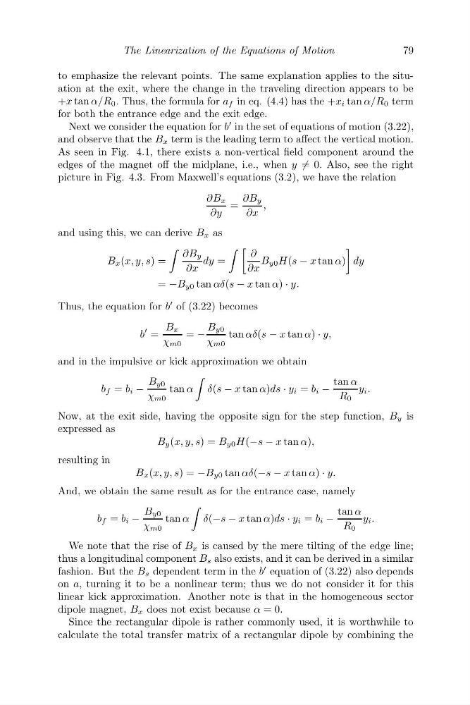
Next we consider the equation for b
in the set of equations of motion (3.22),
and observe that the B x term is the leading term to affect the vertical motion.
As seen in Fig. 4.1, there exists a non-vertical field component around the
edges of the magnet off the midplane, i.e., when y = 0. Also, see the right
picture in Fig. 4.3. From Maxwell’s equations (3.2), we have the relation
∂B x
∂y
=
∂B y
∂x
,
and using this, we can derive B x as
B x (x, y, s) =
∂B y
∂x
dy =
∂
∂x
B y0 H(s − x tan α)
dy
= −B y0 tan αδ(s − x tan α) · y.
Thus, the equation for b
of (3.22) becomes
b
=
B x
χ m0
= −
B y0
χ m0
tan αδ(s − x tan α) · y,
and in the impulsive or kick approximation we obtain
b f = b i −
B y0
χ m0
tan α
δ(s − x tan α)ds · y i = b i −
tan α
R 0
y i .
Now, at the exit side, having the opposite sign for the step function, B y is
expressed as
B y (x, y, s) = B y0 H(−s − x tan α),
resulting in
B x (x, y, s) = −B y0 tan αδ(−s − x tan α) · y.
And, we obtain the same result as for the entrance case, namely
b f = b i −
B y0
χ m0
tan α
δ(−s − x tan α)ds · y i = b i −
tan α
R 0
y i .
We note that the rise of B x is caused by the mere tilting of the edge line;
thus a longitudinal component B s also exists, and it can be derived in a similar
fashion. But the B s dependent term in the b
equation of (3.22) also depends
on a, turning it to be a nonlinear term; thus we do not consider it for this
linear kick approximation. Another note is that in the homogeneous sector
dipole magnet, B x does not exist because α = 0.
Since the rectangular dipole is rather commonly used, it is worthwhile to
calculate the total transfer matrix of a rectangular dipole by combining the
79
to emphasize the relevant points. The same explanation applies to the situation at the exit, where the change in the traveling direction appears to be
+x tan α/R 0 . Thus, the formula for a f in eq. (4.4) has the +x i tan α/R 0 term
for both the entrance edge and the exit edge.
Next we consider the equation for b
in the set of equations of motion (3.22),
and observe that the B x term is the leading term to affect the vertical motion.
As seen in Fig. 4.1, there exists a non-vertical field component around the
edges of the magnet off the midplane, i.e., when y = 0. Also, see the right
picture in Fig. 4.3. From Maxwell’s equations (3.2), we have the relation
∂B x
∂y
=
∂B y
∂x
,
and using this, we can derive B x as
B x (x, y, s) =
∂B y
∂x
dy =
∂
∂x
B y0 H(s − x tan α)
dy
= −B y0 tan αδ(s − x tan α) · y.
Thus, the equation for b
of (3.22) becomes
b
=
B x
χ m0
= −
B y0
χ m0
tan αδ(s − x tan α) · y,
and in the impulsive or kick approximation we obtain
b f = b i −
B y0
χ m0
tan α
δ(s − x tan α)ds · y i = b i −
tan α
R 0
y i .
Now, at the exit side, having the opposite sign for the step function, B y is
expressed as
B y (x, y, s) = B y0 H(−s − x tan α),
resulting in
B x (x, y, s) = −B y0 tan αδ(−s − x tan α) · y.
And, we obtain the same result as for the entrance case, namely
b f = b i −
B y0
χ m0
tan α
δ(−s − x tan α)ds · y i = b i −
tan α
R 0
y i .
We note that the rise of B x is caused by the mere tilting of the edge line;
thus a longitudinal component B s also exists, and it can be derived in a similar
fashion. But the B s dependent term in the b
equation of (3.22) also depends
on a, turning it to be a nonlinear term; thus we do not consider it for this
linear kick approximation. Another note is that in the homogeneous sector
dipole magnet, B x does not exist because α = 0.
Since the rectangular dipole is rather commonly used, it is worthwhile to
calculate the total transfer matrix of a rectangular dipole by combining the