

78
An Introduction to Beam Physics
V
[WDQ
[
α
5
\
V[WDQ α
%\
β
[
α
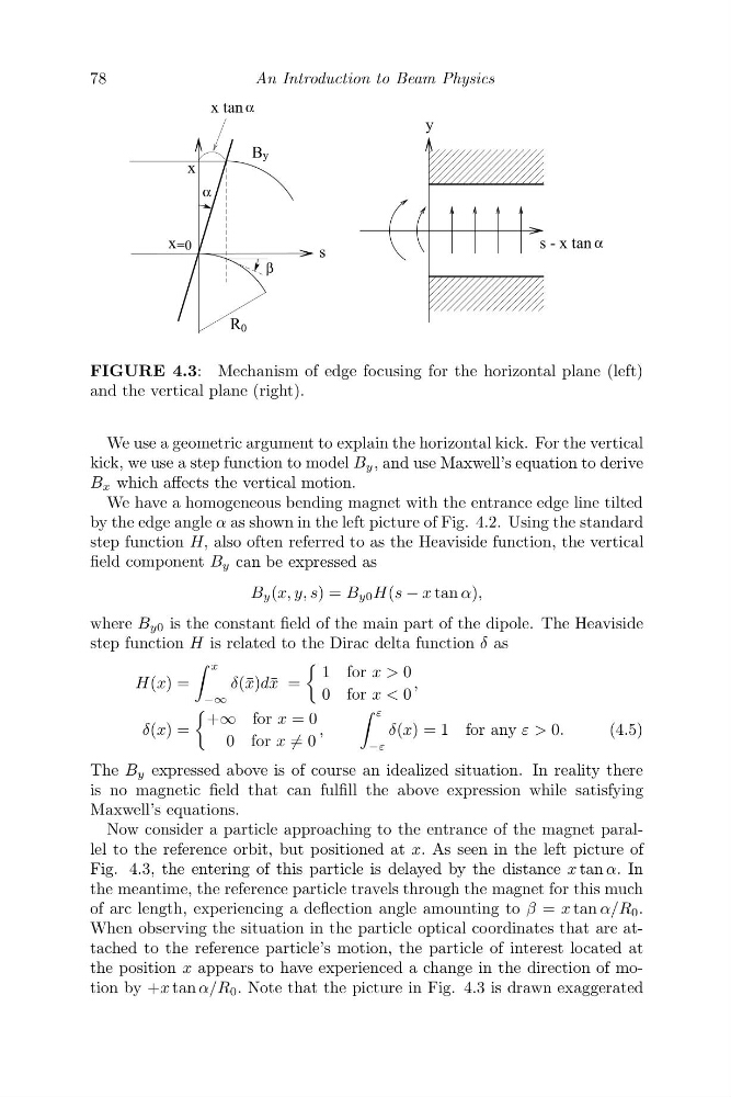
FIGURE 4.3: Mechanism of edge focusing for the horizontal plane (left)
and the vertical plane (right).
We use a geometric argument to explain the horizontal kick. For the vertical
kick, we use a step function to model B y , and use Maxwell’s equation to derive
B x which affects the vertical motion.
We have a homogeneous bending magnet with the entrance edge line tilted
by the edge angle α as shown in the left picture of Fig. 4.2. Using the standard
step function H, also often referred to as the Heaviside function, the vertical
field component B y can be expressed as
B y (x, y, s) = B y0 H(s − x tan α),
where B y0 is the constant field of the main part of the dipole. The Heaviside
step function H is related to the Dirac delta function δ as
H(x) =
x
−∞
δ(¯ x)d¯ x =
1 for x > 0
0 for x < 0
,
δ(x) =
+∞ for x = 0
0 for x = 0
,
ε
−ε
δ(x) = 1 for any ε > 0.
(4.5)
The B y expressed above is of course an idealized situation. In reality there
is no magnetic field that can fulfill the above expression while satisfying
Maxwell’s equations.
Now consider a particle approaching to the entrance of the magnet parallel to the reference orbit, but positioned at x. As seen in the left picture of
Fig. 4.3, the entering of this particle is delayed by the distance x tan α. In
the meantime, the reference particle travels through the magnet for this much
of arc length, experiencing a deflection angle amounting to β = x tan α/R 0 .
When observing the situation in the particle optical coordinates that are attached to the reference particle’s motion, the particle of interest located at
the position x appears to have experienced a change in the direction of motion by +x tan α/R 0 . Note that the picture in Fig. 4.3 is drawn exaggerated
An Introduction to Beam Physics
V
[WDQ
[
α
5
\
V[WDQ α
%\
β
[
α
FIGURE 4.3: Mechanism of edge focusing for the horizontal plane (left)
and the vertical plane (right).
We use a geometric argument to explain the horizontal kick. For the vertical
kick, we use a step function to model B y , and use Maxwell’s equation to derive
B x which affects the vertical motion.
We have a homogeneous bending magnet with the entrance edge line tilted
by the edge angle α as shown in the left picture of Fig. 4.2. Using the standard
step function H, also often referred to as the Heaviside function, the vertical
field component B y can be expressed as
B y (x, y, s) = B y0 H(s − x tan α),
where B y0 is the constant field of the main part of the dipole. The Heaviside
step function H is related to the Dirac delta function δ as
H(x) =
x
−∞
δ(¯ x)d¯ x =
1 for x > 0
0 for x < 0
,
δ(x) =
+∞ for x = 0
0 for x = 0
,
ε
−ε
δ(x) = 1 for any ε > 0.
(4.5)
The B y expressed above is of course an idealized situation. In reality there
is no magnetic field that can fulfill the above expression while satisfying
Maxwell’s equations.
Now consider a particle approaching to the entrance of the magnet parallel to the reference orbit, but positioned at x. As seen in the left picture of
Fig. 4.3, the entering of this particle is delayed by the distance x tan α. In
the meantime, the reference particle travels through the magnet for this much
of arc length, experiencing a deflection angle amounting to β = x tan α/R 0 .
When observing the situation in the particle optical coordinates that are attached to the reference particle’s motion, the particle of interest located at
the position x appears to have experienced a change in the direction of motion by +x tan α/R 0 . Note that the picture in Fig. 4.3 is drawn exaggerated